colRowRanges
matrixStats: Benchmark report
This report benchmark the performance of colRanges() and rowRanges() against alternative methods.
- apply() + range()
> rmatrix <- function(nrow, ncol, mode = c("logical", "double", "integer", "index"), range = c(-100,
+     +100), na_prob = 0) {
+     mode <- match.arg(mode)
+     n <- nrow * ncol
+     if (mode == "logical") {
+         x <- sample(c(FALSE, TRUE), size = n, replace = TRUE)
+     }     else if (mode == "index") {
+         x <- seq_len(n)
+         mode <- "integer"
+     }     else {
+         x <- runif(n, min = range[1], max = range[2])
+     }
+     storage.mode(x) <- mode
+     if (na_prob > 0)
+         x[sample(n, size = na_prob * n)] <- NA
+     dim(x) <- c(nrow, ncol)
+     x
+ }
> rmatrices <- function(scale = 10, seed = 1, ...) {
+     set.seed(seed)
+     data <- list()
+     data[[1]] <- rmatrix(nrow = scale * 1, ncol = scale * 1, ...)
+     data[[2]] <- rmatrix(nrow = scale * 10, ncol = scale * 10, ...)
+     data[[3]] <- rmatrix(nrow = scale * 100, ncol = scale * 1, ...)
+     data[[4]] <- t(data[[3]])
+     data[[5]] <- rmatrix(nrow = scale * 10, ncol = scale * 100, ...)
+     data[[6]] <- t(data[[5]])
+     names(data) <- sapply(data, FUN = function(x) paste(dim(x), collapse = "x"))
+     data
+ }
> data <- rmatrices(mode = mode)> X <- data[["10x10"]]
> gc()
used (Mb) gc trigger (Mb) max used (Mb)
Ncells 3185955 170.2 5709258 305.0 5709258 305.0
Vcells 6413357 49.0 22343563 170.5 56666022 432.4
> colStats <- microbenchmark(colRanges = colRanges(X, na.rm = FALSE), `apply+range` = apply(X, MARGIN = 2L,
+ FUN = range, na.rm = FALSE), unit = "ms")
> X <- t(X)
> gc()
used (Mb) gc trigger (Mb) max used (Mb)
Ncells 3184275 170.1 5709258 305.0 5709258 305.0
Vcells 6408445 48.9 22343563 170.5 56666022 432.4
> rowStats <- microbenchmark(rowRanges = rowRanges(X, na.rm = FALSE), `apply+range` = apply(X, MARGIN = 1L,
+ FUN = range, na.rm = FALSE), unit = "ms")Table: Benchmarking of colRanges() and apply+range() on integer+10x10 data. The top panel shows times in milliseconds and the bottom panel shows relative times.
| expr | min | lq | mean | median | uq | max | |
|---|---|---|---|---|---|---|---|
| 1 | colRanges | 0.001188 | 0.0013595 | 0.0017808 | 0.0015495 | 0.002058 | 0.009749 |
| 2 | apply+range | 0.036074 | 0.0369740 | 0.0384891 | 0.0374310 | 0.037765 | 0.112069 |
| expr | min | lq | mean | median | uq | max | |
|---|---|---|---|---|---|---|---|
| 1 | colRanges | 1.00000 | 1.00000 | 1.00000 | 1.00000 | 1.00000 | 1.00000 |
| 2 | apply+range | 30.36532 | 27.19676 | 21.61363 | 24.15682 | 18.35034 | 11.49544 |
Table: Benchmarking of rowRanges() and apply+range() on integer+10x10 data (transposed). The top panel shows times in milliseconds and the bottom panel shows relative times.
| expr | min | lq | mean | median | uq | max | |
|---|---|---|---|---|---|---|---|
| 1 | rowRanges | 0.001189 | 0.0014305 | 0.0019098 | 0.001948 | 0.0020940 | 0.011684 |
| 2 | apply+range | 0.036328 | 0.0372705 | 0.0391010 | 0.037737 | 0.0383145 | 0.145866 |
| expr | min | lq | mean | median | uq | max | |
|---|---|---|---|---|---|---|---|
| 1 | rowRanges | 1.00000 | 1.00000 | 1.00000 | 1.00000 | 1.00000 | 1.00000 |
| 2 | apply+range | 30.55341 | 26.05418 | 20.47367 | 19.37218 | 18.29728 | 12.48425 |
Figure: Benchmarking of colRanges() and apply+range() on integer+10x10 data as well as rowRanges() and apply+range() on the same data transposed. Outliers are displayed as crosses. Times are in milliseconds.

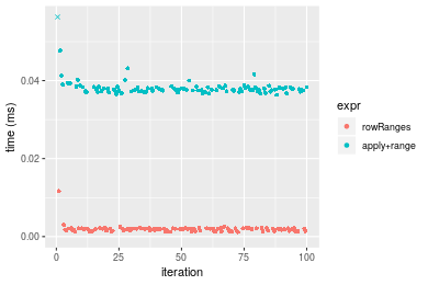 Table: Benchmarking of colRanges() and rowRanges() on integer+10x10 data (original and transposed). The top panel shows times in milliseconds and the bottom panel shows relative times.
| expr | min | lq | mean | median | uq | max | |
|---|---|---|---|---|---|---|---|
| 1 | colRanges | 1.188 | 1.3595 | 1.78078 | 1.5495 | 2.058 | 9.749 |
| 2 | rowRanges | 1.189 | 1.4305 | 1.90982 | 1.9480 | 2.094 | 11.684 |
| expr | min | lq | mean | median | uq | max | |
|---|---|---|---|---|---|---|---|
| 1 | colRanges | 1.000000 | 1.000000 | 1.000000 | 1.00000 | 1.000000 | 1.000000 |
| 2 | rowRanges | 1.000842 | 1.052225 | 1.072463 | 1.25718 | 1.017493 | 1.198482 |
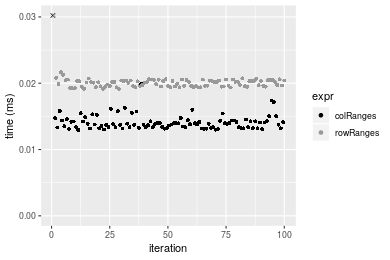
Figure: Benchmarking of colRanges() and rowRanges() on integer+10x10 data (original and transposed). Outliers are displayed as crosses. Times are in milliseconds.

> X <- data[["100x100"]]
> gc()
          used (Mb) gc trigger  (Mb) max used  (Mb)
Ncells 3182828  170    5709258 305.0  5709258 305.0
Vcells 6024946   46   22343563 170.5 56666022 432.4
> colStats <- microbenchmark(colRanges = colRanges(X, na.rm = FALSE), `apply+range` = apply(X, MARGIN = 2L,
+     FUN = range, na.rm = FALSE), unit = "ms")
> X <- t(X)
> gc()
          used  (Mb) gc trigger  (Mb) max used  (Mb)
Ncells 3182822 170.0    5709258 305.0  5709258 305.0
Vcells 6029989  46.1   22343563 170.5 56666022 432.4
> rowStats <- microbenchmark(rowRanges = rowRanges(X, na.rm = FALSE), `apply+range` = apply(X, MARGIN = 1L,
+     FUN = range, na.rm = FALSE), unit = "ms")
Table: Benchmarking of colRanges() and apply+range() on integer+100x100 data. The top panel shows times in milliseconds and the bottom panel shows relative times.
| expr | min | lq | mean | median | uq | max | |
|---|---|---|---|---|---|---|---|
| 1 | colRanges | 0.019493 | 0.0204015 | 0.0211931 | 0.021145 | 0.0216250 | 0.034272 |
| 2 | apply+range | 0.286671 | 0.2895970 | 0.2955994 | 0.291265 | 0.2943575 | 0.418665 |
| expr | min | lq | mean | median | uq | max | |
|---|---|---|---|---|---|---|---|
| 1 | colRanges | 1.00000 | 1.00000 | 1.00000 | 1.00000 | 1.00000 | 1.00000 |
| 2 | apply+range | 14.70636 | 14.19489 | 13.94793 | 13.77465 | 13.61191 | 12.21595 |
Table: Benchmarking of rowRanges() and apply+range() on integer+100x100 data (transposed). The top panel shows times in milliseconds and the bottom panel shows relative times.
| expr | min | lq | mean | median | uq | max | |
|---|---|---|---|---|---|---|---|
| 1 | rowRanges | 0.019008 | 0.0200585 | 0.0208961 | 0.0207775 | 0.021445 | 0.032492 |
| 2 | apply+range | 0.289331 | 0.2915570 | 0.2983378 | 0.2932490 | 0.296419 | 0.470623 |
| expr | min | lq | mean | median | uq | max | |
|---|---|---|---|---|---|---|---|
| 1 | rowRanges | 1.00000 | 1.00000 | 1.00000 | 1.00000 | 1.00000 | 1.00000 |
| 2 | apply+range | 15.22154 | 14.53533 | 14.27718 | 14.11378 | 13.82229 | 14.48427 |
Figure: Benchmarking of colRanges() and apply+range() on integer+100x100 data as well as rowRanges() and apply+range() on the same data transposed. Outliers are displayed as crosses. Times are in milliseconds.

 Table: Benchmarking of colRanges() and rowRanges() on integer+100x100 data (original and transposed). The top panel shows times in milliseconds and the bottom panel shows relative times.
| expr | min | lq | mean | median | uq | max | |
|---|---|---|---|---|---|---|---|
| 2 | rowRanges | 19.008 | 20.0585 | 20.89613 | 20.7775 | 21.445 | 32.492 |
| 1 | colRanges | 19.493 | 20.4015 | 21.19306 | 21.1450 | 21.625 | 34.272 |
| expr | min | lq | mean | median | uq | max | |
|---|---|---|---|---|---|---|---|
| 2 | rowRanges | 1.000000 | 1.0000 | 1.00000 | 1.000000 | 1.000000 | 1.000000 |
| 1 | colRanges | 1.025516 | 1.0171 | 1.01421 | 1.017687 | 1.008394 | 1.054783 |
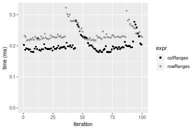
Figure: Benchmarking of colRanges() and rowRanges() on integer+100x100 data (original and transposed). Outliers are displayed as crosses. Times are in milliseconds.

> X <- data[["1000x10"]]
> gc()
          used  (Mb) gc trigger  (Mb) max used  (Mb)
Ncells 3183561 170.1    5709258 305.0  5709258 305.0
Vcells 6028466  46.0   22343563 170.5 56666022 432.4
> colStats <- microbenchmark(colRanges = colRanges(X, na.rm = FALSE), `apply+range` = apply(X, MARGIN = 2L,
+     FUN = range, na.rm = FALSE), unit = "ms")
> X <- t(X)
> gc()
          used  (Mb) gc trigger  (Mb) max used  (Mb)
Ncells 3183552 170.1    5709258 305.0  5709258 305.0
Vcells 6033504  46.1   22343563 170.5 56666022 432.4
> rowStats <- microbenchmark(rowRanges = rowRanges(X, na.rm = FALSE), `apply+range` = apply(X, MARGIN = 1L,
+     FUN = range, na.rm = FALSE), unit = "ms")
Table: Benchmarking of colRanges() and apply+range() on integer+1000x10 data. The top panel shows times in milliseconds and the bottom panel shows relative times.
| expr | min | lq | mean | median | uq | max | |
|---|---|---|---|---|---|---|---|
| 1 | colRanges | 0.014935 | 0.0152270 | 0.0157857 | 0.0157040 | 0.0158965 | 0.030208 |
| 2 | apply+range | 0.109673 | 0.1113615 | 0.1147352 | 0.1141055 | 0.1150540 | 0.192582 |
| expr | min | lq | mean | median | uq | max | |
|---|---|---|---|---|---|---|---|
| 1 | colRanges | 1.000000 | 1.000000 | 1.000000 | 1.000000 | 1.000000 | 1.000000 |
| 2 | apply+range | 7.343355 | 7.313423 | 7.268316 | 7.266015 | 7.237694 | 6.375199 |
Table: Benchmarking of rowRanges() and apply+range() on integer+1000x10 data (transposed). The top panel shows times in milliseconds and the bottom panel shows relative times.
| expr | min | lq | mean | median | uq | max | |
|---|---|---|---|---|---|---|---|
| 1 | rowRanges | 0.016718 | 0.0171375 | 0.0177167 | 0.017611 | 0.017921 | 0.031567 |
| 2 | apply+range | 0.109371 | 0.1112560 | 0.1151728 | 0.114329 | 0.115622 | 0.192081 |
| expr | min | lq | mean | median | uq | max | |
|---|---|---|---|---|---|---|---|
| 1 | rowRanges | 1.00000 | 1.000000 | 1.000000 | 1.000000 | 1.00000 | 1.000000 |
| 2 | apply+range | 6.54211 | 6.491962 | 6.500791 | 6.491909 | 6.45176 | 6.084867 |
Figure: Benchmarking of colRanges() and apply+range() on integer+1000x10 data as well as rowRanges() and apply+range() on the same data transposed. Outliers are displayed as crosses. Times are in milliseconds.

 Table: Benchmarking of colRanges() and rowRanges() on integer+1000x10 data (original and transposed). The top panel shows times in milliseconds and the bottom panel shows relative times.
| expr | min | lq | mean | median | uq | max | |
|---|---|---|---|---|---|---|---|
| 1 | colRanges | 14.935 | 15.2270 | 15.78566 | 15.704 | 15.8965 | 30.208 |
| 2 | rowRanges | 16.718 | 17.1375 | 17.71674 | 17.611 | 17.9210 | 31.567 |
| expr | min | lq | mean | median | uq | max | |
|---|---|---|---|---|---|---|---|
| 1 | colRanges | 1.000000 | 1.000000 | 1.000000 | 1.000000 | 1.000000 | 1.000000 |
| 2 | rowRanges | 1.119384 | 1.125468 | 1.122331 | 1.121434 | 1.127355 | 1.044988 |
Figure: Benchmarking of colRanges() and rowRanges() on integer+1000x10 data (original and transposed). Outliers are displayed as crosses. Times are in milliseconds.

> X <- data[["10x1000"]]
> gc()
          used  (Mb) gc trigger  (Mb) max used  (Mb)
Ncells 3183746 170.1    5709258 305.0  5709258 305.0
Vcells 6029138  46.0   22343563 170.5 56666022 432.4
> colStats <- microbenchmark(colRanges = colRanges(X, na.rm = FALSE), `apply+range` = apply(X, MARGIN = 2L,
+     FUN = range, na.rm = FALSE), unit = "ms")
> X <- t(X)
> gc()
          used  (Mb) gc trigger  (Mb) max used  (Mb)
Ncells 3183740 170.1    5709258 305.0  5709258 305.0
Vcells 6034181  46.1   22343563 170.5 56666022 432.4
> rowStats <- microbenchmark(rowRanges = rowRanges(X, na.rm = FALSE), `apply+range` = apply(X, MARGIN = 1L,
+     FUN = range, na.rm = FALSE), unit = "ms")
Table: Benchmarking of colRanges() and apply+range() on integer+10x1000 data. The top panel shows times in milliseconds and the bottom panel shows relative times.
| expr | min | lq | mean | median | uq | max | |
|---|---|---|---|---|---|---|---|
| 1 | colRanges | 0.043947 | 0.045743 | 0.0474114 | 0.0472785 | 0.048195 | 0.061508 |
| 2 | apply+range | 1.967796 | 2.010960 | 2.1402157 | 2.0420700 | 2.140857 | 7.481601 |
| expr | min | lq | mean | median | uq | max | |
|---|---|---|---|---|---|---|---|
| 1 | colRanges | 1.00000 | 1.00000 | 1.00000 | 1.00000 | 1.00000 | 1.0000 |
| 2 | apply+range | 44.77657 | 43.96214 | 45.14138 | 43.19236 | 44.42073 | 121.6362 |
Table: Benchmarking of rowRanges() and apply+range() on integer+10x1000 data (transposed). The top panel shows times in milliseconds and the bottom panel shows relative times.
| expr | min | lq | mean | median | uq | max | |
|---|---|---|---|---|---|---|---|
| 1 | rowRanges | 0.041714 | 0.0435925 | 0.0460086 | 0.0449345 | 0.046621 | 0.106088 |
| 2 | apply+range | 1.946157 | 1.9968740 | 2.1388868 | 2.0386435 | 2.138240 | 7.513914 |
| expr | min | lq | mean | median | uq | max | |
|---|---|---|---|---|---|---|---|
| 1 | rowRanges | 1.00000 | 1.00000 | 1.00000 | 1.00000 | 1.0000 | 1.00000 |
| 2 | apply+range | 46.65477 | 45.80774 | 46.48884 | 45.36923 | 45.8643 | 70.82718 |
Figure: Benchmarking of colRanges() and apply+range() on integer+10x1000 data as well as rowRanges() and apply+range() on the same data transposed. Outliers are displayed as crosses. Times are in milliseconds.

 Table: Benchmarking of colRanges() and rowRanges() on integer+10x1000 data (original and transposed). The top panel shows times in milliseconds and the bottom panel shows relative times.
| expr | min | lq | mean | median | uq | max | |
|---|---|---|---|---|---|---|---|
| 2 | rowRanges | 41.714 | 43.5925 | 46.00861 | 44.9345 | 46.621 | 106.088 |
| 1 | colRanges | 43.947 | 45.7430 | 47.41139 | 47.2785 | 48.195 | 61.508 |
| expr | min | lq | mean | median | uq | max | |
|---|---|---|---|---|---|---|---|
| 2 | rowRanges | 1.000000 | 1.000000 | 1.00000 | 1.000000 | 1.000000 | 1.0000000 |
| 1 | colRanges | 1.053531 | 1.049332 | 1.03049 | 1.052165 | 1.033762 | 0.5797828 |
Figure: Benchmarking of colRanges() and rowRanges() on integer+10x1000 data (original and transposed). Outliers are displayed as crosses. Times are in milliseconds.

> X <- data[["100x1000"]]
> gc()
          used  (Mb) gc trigger  (Mb) max used  (Mb)
Ncells 3183930 170.1    5709258 305.0  5709258 305.0
Vcells 6029621  46.1   22343563 170.5 56666022 432.4
> colStats <- microbenchmark(colRanges = colRanges(X, na.rm = FALSE), `apply+range` = apply(X, MARGIN = 2L,
+     FUN = range, na.rm = FALSE), unit = "ms")
> X <- t(X)
> gc()
          used  (Mb) gc trigger  (Mb) max used  (Mb)
Ncells 3183924 170.1    5709258 305.0  5709258 305.0
Vcells 6079664  46.4   22343563 170.5 56666022 432.4
> rowStats <- microbenchmark(rowRanges = rowRanges(X, na.rm = FALSE), `apply+range` = apply(X, MARGIN = 1L,
+     FUN = range, na.rm = FALSE), unit = "ms")
Table: Benchmarking of colRanges() and apply+range() on integer+100x1000 data. The top panel shows times in milliseconds and the bottom panel shows relative times.
| expr | min | lq | mean | median | uq | max | |
|---|---|---|---|---|---|---|---|
| 1 | colRanges | 0.195850 | 0.1981605 | 0.2072418 | 0.2039755 | 0.2098685 | 0.258956 |
| 2 | apply+range | 2.683579 | 2.7374205 | 2.9877983 | 2.8024365 | 2.8899875 | 17.625025 |
| expr | min | lq | mean | median | uq | max | |
|---|---|---|---|---|---|---|---|
| 1 | colRanges | 1.00000 | 1.00000 | 1.00000 | 1.00000 | 1.00000 | 1.00000 |
| 2 | apply+range | 13.70222 | 13.81416 | 14.41697 | 13.73908 | 13.77047 | 68.06185 |
Table: Benchmarking of rowRanges() and apply+range() on integer+100x1000 data (transposed). The top panel shows times in milliseconds and the bottom panel shows relative times.
| expr | min | lq | mean | median | uq | max | |
|---|---|---|---|---|---|---|---|
| 1 | rowRanges | 0.190614 | 0.194564 | 0.2014488 | 0.201166 | 0.203994 | 0.249796 |
| 2 | apply+range | 2.687045 | 2.764858 | 3.0294722 | 2.848991 | 2.915337 | 18.072235 |
| expr | min | lq | mean | median | uq | max | |
|---|---|---|---|---|---|---|---|
| 1 | rowRanges | 1.00000 | 1.00000 | 1.00000 | 1.00000 | 1.00000 | 1.00000 |
| 2 | apply+range | 14.09679 | 14.21053 | 15.03842 | 14.16239 | 14.29129 | 72.34798 |
Figure: Benchmarking of colRanges() and apply+range() on integer+100x1000 data as well as rowRanges() and apply+range() on the same data transposed. Outliers are displayed as crosses. Times are in milliseconds.

 Table: Benchmarking of colRanges() and rowRanges() on integer+100x1000 data (original and transposed). The top panel shows times in milliseconds and the bottom panel shows relative times.
| expr | min | lq | mean | median | uq | max | |
|---|---|---|---|---|---|---|---|
| 2 | rowRanges | 190.614 | 194.5640 | 201.4488 | 201.1660 | 203.9940 | 249.796 |
| 1 | colRanges | 195.850 | 198.1605 | 207.2418 | 203.9755 | 209.8685 | 258.956 |
| expr | min | lq | mean | median | uq | max | |
|---|---|---|---|---|---|---|---|
| 2 | rowRanges | 1.000000 | 1.000000 | 1.000000 | 1.000000 | 1.000000 | 1.00000 |
| 1 | colRanges | 1.027469 | 1.018485 | 1.028757 | 1.013966 | 1.028797 | 1.03667 |
Figure: Benchmarking of colRanges() and rowRanges() on integer+100x1000 data (original and transposed). Outliers are displayed as crosses. Times are in milliseconds.

> X <- data[["1000x100"]]
> gc()
          used  (Mb) gc trigger  (Mb) max used  (Mb)
Ncells 3184122 170.1    5709258 305.0  5709258 305.0
Vcells 6030183  46.1   22343563 170.5 56666022 432.4
> colStats <- microbenchmark(colRanges = colRanges(X, na.rm = FALSE), `apply+range` = apply(X, MARGIN = 2L,
+     FUN = range, na.rm = FALSE), unit = "ms")
> X <- t(X)
> gc()
          used  (Mb) gc trigger  (Mb) max used  (Mb)
Ncells 3184116 170.1    5709258 305.0  5709258 305.0
Vcells 6080226  46.4   22343563 170.5 56666022 432.4
> rowStats <- microbenchmark(rowRanges = rowRanges(X, na.rm = FALSE), `apply+range` = apply(X, MARGIN = 1L,
+     FUN = range, na.rm = FALSE), unit = "ms")
Table: Benchmarking of colRanges() and apply+range() on integer+1000x100 data. The top panel shows times in milliseconds and the bottom panel shows relative times.
| expr | min | lq | mean | median | uq | max | |
|---|---|---|---|---|---|---|---|
| 1 | colRanges | 0.141058 | 0.1422235 | 0.1504843 | 0.1427965 | 0.1485420 | 0.192611 |
| 2 | apply+range | 0.902127 | 0.9093035 | 1.0440243 | 0.9193610 | 0.9761505 | 9.368515 |
| expr | min | lq | mean | median | uq | max | |
|---|---|---|---|---|---|---|---|
| 1 | colRanges | 1.000000 | 1.000000 | 1.000000 | 1.00000 | 1.000000 | 1.00000 |
| 2 | apply+range | 6.395433 | 6.393483 | 6.937761 | 6.43826 | 6.571545 | 48.63956 |
Table: Benchmarking of rowRanges() and apply+range() on integer+1000x100 data (transposed). The top panel shows times in milliseconds and the bottom panel shows relative times.
| expr | min | lq | mean | median | uq | max | |
|---|---|---|---|---|---|---|---|
| 1 | rowRanges | 0.149136 | 0.150664 | 0.1591479 | 0.153410 | 0.156948 | 0.203205 |
| 2 | apply+range | 0.909309 | 0.942989 | 1.0766903 | 0.957465 | 0.996298 | 9.315277 |
| expr | min | lq | mean | median | uq | max | |
|---|---|---|---|---|---|---|---|
| 1 | rowRanges | 1.00000 | 1.000000 | 1.000000 | 1.000000 | 1.00000 | 1.00000 |
| 2 | apply+range | 6.09718 | 6.258887 | 6.765345 | 6.241216 | 6.34795 | 45.84177 |
Figure: Benchmarking of colRanges() and apply+range() on integer+1000x100 data as well as rowRanges() and apply+range() on the same data transposed. Outliers are displayed as crosses. Times are in milliseconds.

 Table: Benchmarking of colRanges() and rowRanges() on integer+1000x100 data (original and transposed). The top panel shows times in milliseconds and the bottom panel shows relative times.
| expr | min | lq | mean | median | uq | max | |
|---|---|---|---|---|---|---|---|
| 1 | colRanges | 141.058 | 142.2235 | 150.4843 | 142.7965 | 148.542 | 192.611 |
| 2 | rowRanges | 149.136 | 150.6640 | 159.1479 | 153.4100 | 156.948 | 203.205 |
| expr | min | lq | mean | median | uq | max | |
|---|---|---|---|---|---|---|---|
| 1 | colRanges | 1.000000 | 1.000000 | 1.000000 | 1.000000 | 1.00000 | 1.000000 |
| 2 | rowRanges | 1.057267 | 1.059347 | 1.057571 | 1.074326 | 1.05659 | 1.055002 |
Figure: Benchmarking of colRanges() and rowRanges() on integer+1000x100 data (original and transposed). Outliers are displayed as crosses. Times are in milliseconds.

> rmatrix <- function(nrow, ncol, mode = c("logical", "double", "integer", "index"), range = c(-100,
+     +100), na_prob = 0) {
+     mode <- match.arg(mode)
+     n <- nrow * ncol
+     if (mode == "logical") {
+         x <- sample(c(FALSE, TRUE), size = n, replace = TRUE)
+     }     else if (mode == "index") {
+         x <- seq_len(n)
+         mode <- "integer"
+     }     else {
+         x <- runif(n, min = range[1], max = range[2])
+     }
+     storage.mode(x) <- mode
+     if (na_prob > 0)
+         x[sample(n, size = na_prob * n)] <- NA
+     dim(x) <- c(nrow, ncol)
+     x
+ }
> rmatrices <- function(scale = 10, seed = 1, ...) {
+     set.seed(seed)
+     data <- list()
+     data[[1]] <- rmatrix(nrow = scale * 1, ncol = scale * 1, ...)
+     data[[2]] <- rmatrix(nrow = scale * 10, ncol = scale * 10, ...)
+     data[[3]] <- rmatrix(nrow = scale * 100, ncol = scale * 1, ...)
+     data[[4]] <- t(data[[3]])
+     data[[5]] <- rmatrix(nrow = scale * 10, ncol = scale * 100, ...)
+     data[[6]] <- t(data[[5]])
+     names(data) <- sapply(data, FUN = function(x) paste(dim(x), collapse = "x"))
+     data
+ }
> data <- rmatrices(mode = mode)> X <- data[["10x10"]]
> gc()
used (Mb) gc trigger (Mb) max used (Mb)
Ncells 3184330 170.1 5709258 305.0 5709258 305.0
Vcells 6146532 46.9 22343563 170.5 56666022 432.4
> colStats <- microbenchmark(colRanges = colRanges(X, na.rm = FALSE), `apply+range` = apply(X, MARGIN = 2L,
+ FUN = range, na.rm = FALSE), unit = "ms")
> X <- t(X)
> gc()
used (Mb) gc trigger (Mb) max used (Mb)
Ncells 3184315 170.1 5709258 305.0 5709258 305.0
Vcells 6146660 46.9 22343563 170.5 56666022 432.4
> rowStats <- microbenchmark(rowRanges = rowRanges(X, na.rm = FALSE), `apply+range` = apply(X, MARGIN = 1L,
+ FUN = range, na.rm = FALSE), unit = "ms")Table: Benchmarking of colRanges() and apply+range() on double+10x10 data. The top panel shows times in milliseconds and the bottom panel shows relative times.
| expr | min | lq | mean | median | uq | max | |
|---|---|---|---|---|---|---|---|
| 1 | colRanges | 0.001233 | 0.0015645 | 0.002038 | 0.0019235 | 0.0022495 | 0.010014 |
| 2 | apply+range | 0.036716 | 0.0382100 | 0.039597 | 0.0386610 | 0.0392060 | 0.117575 |
| expr | min | lq | mean | median | uq | max | |
|---|---|---|---|---|---|---|---|
| 1 | colRanges | 1.00000 | 1.00000 | 1.00000 | 1.0000 | 1.00000 | 1.00000 |
| 2 | apply+range | 29.77778 | 24.42314 | 19.42906 | 20.0993 | 17.42876 | 11.74106 |
Table: Benchmarking of rowRanges() and apply+range() on double+10x10 data (transposed). The top panel shows times in milliseconds and the bottom panel shows relative times.
| expr | min | lq | mean | median | uq | max | |
|---|---|---|---|---|---|---|---|
| 1 | rowRanges | 0.001226 | 0.001625 | 0.0021325 | 0.0021420 | 0.002341 | 0.010143 |
| 2 | apply+range | 0.036255 | 0.037761 | 0.0391419 | 0.0381995 | 0.038659 | 0.111980 |
| expr | min | lq | mean | median | uq | max | |
|---|---|---|---|---|---|---|---|
| 1 | rowRanges | 1.00000 | 1.00000 | 1.00000 | 1.00000 | 1.00000 | 1.00000 |
| 2 | apply+range | 29.57178 | 23.23754 | 18.35502 | 17.83357 | 16.51388 | 11.04013 |
Figure: Benchmarking of colRanges() and apply+range() on double+10x10 data as well as rowRanges() and apply+range() on the same data transposed. Outliers are displayed as crosses. Times are in milliseconds.

 Table: Benchmarking of colRanges() and rowRanges() on double+10x10 data (original and transposed). The top panel shows times in milliseconds and the bottom panel shows relative times.
| expr | min | lq | mean | median | uq | max | |
|---|---|---|---|---|---|---|---|
| 1 | colRanges | 1.233 | 1.5645 | 2.03803 | 1.9235 | 2.2495 | 10.014 |
| 2 | rowRanges | 1.226 | 1.6250 | 2.13249 | 2.1420 | 2.3410 | 10.143 |
| expr | min | lq | mean | median | uq | max | |
|---|---|---|---|---|---|---|---|
| 1 | colRanges | 1.0000000 | 1.000000 | 1.000000 | 1.000000 | 1.000000 | 1.000000 |
| 2 | rowRanges | 0.9943228 | 1.038671 | 1.046349 | 1.113595 | 1.040676 | 1.012882 |
Figure: Benchmarking of colRanges() and rowRanges() on double+10x10 data (original and transposed). Outliers are displayed as crosses. Times are in milliseconds.

> X <- data[["100x100"]]
> gc()
          used  (Mb) gc trigger  (Mb) max used  (Mb)
Ncells 3184510 170.1    5709258 305.0  5709258 305.0
Vcells 6146644  46.9   22343563 170.5 56666022 432.4
> colStats <- microbenchmark(colRanges = colRanges(X, na.rm = FALSE), `apply+range` = apply(X, MARGIN = 2L,
+     FUN = range, na.rm = FALSE), unit = "ms")
> X <- t(X)
> gc()
          used  (Mb) gc trigger  (Mb) max used  (Mb)
Ncells 3184504 170.1    5709258 305.0  5709258 305.0
Vcells 6156687  47.0   22343563 170.5 56666022 432.4
> rowStats <- microbenchmark(rowRanges = rowRanges(X, na.rm = FALSE), `apply+range` = apply(X, MARGIN = 1L,
+     FUN = range, na.rm = FALSE), unit = "ms")
Table: Benchmarking of colRanges() and apply+range() on double+100x100 data. The top panel shows times in milliseconds and the bottom panel shows relative times.
| expr | min | lq | mean | median | uq | max | |
|---|---|---|---|---|---|---|---|
| 1 | colRanges | 0.016974 | 0.0177975 | 0.0190318 | 0.018428 | 0.0191705 | 0.062640 |
| 2 | apply+range | 0.324943 | 0.3326065 | 0.3440279 | 0.337524 | 0.3444030 | 0.504698 |
| expr | min | lq | mean | median | uq | max | |
|---|---|---|---|---|---|---|---|
| 1 | colRanges | 1.00000 | 1.00000 | 1.00000 | 1.00000 | 1.00000 | 1.00000 |
| 2 | apply+range | 19.14357 | 18.68838 | 18.07643 | 18.31582 | 17.96526 | 8.05712 |
Table: Benchmarking of rowRanges() and apply+range() on double+100x100 data (transposed). The top panel shows times in milliseconds and the bottom panel shows relative times.
| expr | min | lq | mean | median | uq | max | |
|---|---|---|---|---|---|---|---|
| 1 | rowRanges | 0.021905 | 0.0226085 | 0.023331 | 0.0231800 | 0.0236245 | 0.032950 |
| 2 | apply+range | 0.286434 | 0.2896050 | 0.296664 | 0.2925475 | 0.2960620 | 0.437018 |
| expr | min | lq | mean | median | uq | max | |
|---|---|---|---|---|---|---|---|
| 1 | rowRanges | 1.00000 | 1.00000 | 1.00000 | 1.00000 | 1.00000 | 1.00000 |
| 2 | apply+range | 13.07619 | 12.80956 | 12.71547 | 12.62069 | 12.53199 | 13.26307 |
Figure: Benchmarking of colRanges() and apply+range() on double+100x100 data as well as rowRanges() and apply+range() on the same data transposed. Outliers are displayed as crosses. Times are in milliseconds.

 Table: Benchmarking of colRanges() and rowRanges() on double+100x100 data (original and transposed). The top panel shows times in milliseconds and the bottom panel shows relative times.
| expr | min | lq | mean | median | uq | max | |
|---|---|---|---|---|---|---|---|
| 1 | colRanges | 16.974 | 17.7975 | 19.03185 | 18.428 | 19.1705 | 62.64 |
| 2 | rowRanges | 21.905 | 22.6085 | 23.33095 | 23.180 | 23.6245 | 32.95 |
| expr | min | lq | mean | median | uq | max | |
|---|---|---|---|---|---|---|---|
| 1 | colRanges | 1.000000 | 1.000000 | 1.00000 | 1.000000 | 1.000000 | 1.0000000 |
| 2 | rowRanges | 1.290503 | 1.270319 | 1.22589 | 1.257869 | 1.232336 | 0.5260217 |
Figure: Benchmarking of colRanges() and rowRanges() on double+100x100 data (original and transposed). Outliers are displayed as crosses. Times are in milliseconds.

> X <- data[["1000x10"]]
> gc()
          used  (Mb) gc trigger  (Mb) max used  (Mb)
Ncells 3184703 170.1    5709258 305.0  5709258 305.0
Vcells 6147533  47.0   22343563 170.5 56666022 432.4
> colStats <- microbenchmark(colRanges = colRanges(X, na.rm = FALSE), `apply+range` = apply(X, MARGIN = 2L,
+     FUN = range, na.rm = FALSE), unit = "ms")
> X <- t(X)
> gc()
          used  (Mb) gc trigger  (Mb) max used  (Mb)
Ncells 3184694 170.1    5709258 305.0  5709258 305.0
Vcells 6157571  47.0   22343563 170.5 56666022 432.4
> rowStats <- microbenchmark(rowRanges = rowRanges(X, na.rm = FALSE), `apply+range` = apply(X, MARGIN = 1L,
+     FUN = range, na.rm = FALSE), unit = "ms")
Table: Benchmarking of colRanges() and apply+range() on double+1000x10 data. The top panel shows times in milliseconds and the bottom panel shows relative times.
| expr | min | lq | mean | median | uq | max | |
|---|---|---|---|---|---|---|---|
| 1 | colRanges | 0.012952 | 0.0133565 | 0.0143408 | 0.0138830 | 0.0143820 | 0.038035 |
| 2 | apply+range | 0.161635 | 0.1642280 | 0.1687233 | 0.1665045 | 0.1690595 | 0.262972 |
| expr | min | lq | mean | median | uq | max | |
|---|---|---|---|---|---|---|---|
| 1 | colRanges | 1.00000 | 1.00000 | 1.00000 | 1.00000 | 1.00000 | 1.000000 |
| 2 | apply+range | 12.47954 | 12.29574 | 11.76522 | 11.99341 | 11.75494 | 6.913948 |
Table: Benchmarking of rowRanges() and apply+range() on double+1000x10 data (transposed). The top panel shows times in milliseconds and the bottom panel shows relative times.
| expr | min | lq | mean | median | uq | max | |
|---|---|---|---|---|---|---|---|
| 1 | rowRanges | 0.019130 | 0.0195665 | 0.0201674 | 0.0201305 | 0.0204175 | 0.035807 |
| 2 | apply+range | 0.120754 | 0.1231620 | 0.1267325 | 0.1247645 | 0.1275775 | 0.209332 |
| expr | min | lq | mean | median | uq | max | |
|---|---|---|---|---|---|---|---|
| 1 | rowRanges | 1.000000 | 1.000000 | 1.000000 | 1.000000 | 1.000000 | 1.00000 |
| 2 | apply+range | 6.312284 | 6.294534 | 6.284044 | 6.197785 | 6.248439 | 5.84612 |
Figure: Benchmarking of colRanges() and apply+range() on double+1000x10 data as well as rowRanges() and apply+range() on the same data transposed. Outliers are displayed as crosses. Times are in milliseconds.

 Table: Benchmarking of colRanges() and rowRanges() on double+1000x10 data (original and transposed). The top panel shows times in milliseconds and the bottom panel shows relative times.
| expr | min | lq | mean | median | uq | max | |
|---|---|---|---|---|---|---|---|
| 1 | colRanges | 12.952 | 13.3565 | 14.34085 | 13.8830 | 14.3820 | 38.035 |
| 2 | rowRanges | 19.130 | 19.5665 | 20.16735 | 20.1305 | 20.4175 | 35.807 |
| expr | min | lq | mean | median | uq | max | |
|---|---|---|---|---|---|---|---|
| 1 | colRanges | 1.000000 | 1.000000 | 1.000000 | 1.000000 | 1.000000 | 1.0000000 |
| 2 | rowRanges | 1.476992 | 1.464942 | 1.406287 | 1.450011 | 1.419657 | 0.9414224 |
Figure: Benchmarking of colRanges() and rowRanges() on double+1000x10 data (original and transposed). Outliers are displayed as crosses. Times are in milliseconds.
> X <- data[["10x1000"]]
> gc()
          used  (Mb) gc trigger  (Mb) max used  (Mb)
Ncells 3184888 170.1    5709258 305.0  5709258 305.0
Vcells 6148557  47.0   22343563 170.5 56666022 432.4
> colStats <- microbenchmark(colRanges = colRanges(X, na.rm = FALSE), `apply+range` = apply(X, MARGIN = 2L,
+     FUN = range, na.rm = FALSE), unit = "ms")
> X <- t(X)
> gc()
          used  (Mb) gc trigger  (Mb) max used  (Mb)
Ncells 3184882 170.1    5709258 305.0  5709258 305.0
Vcells 6158600  47.0   22343563 170.5 56666022 432.4
> rowStats <- microbenchmark(rowRanges = rowRanges(X, na.rm = FALSE), `apply+range` = apply(X, MARGIN = 1L,
+     FUN = range, na.rm = FALSE), unit = "ms")
Table: Benchmarking of colRanges() and apply+range() on double+10x1000 data. The top panel shows times in milliseconds and the bottom panel shows relative times.
| expr | min | lq | mean | median | uq | max | |
|---|---|---|---|---|---|---|---|
| 1 | colRanges | 0.043253 | 0.0467135 | 0.0487173 | 0.048314 | 0.0497255 | 0.068454 |
| 2 | apply+range | 1.879370 | 1.9707360 | 2.1020929 | 2.035511 | 2.1187615 | 7.015015 |
| expr | min | lq | mean | median | uq | max | |
|---|---|---|---|---|---|---|---|
| 1 | colRanges | 1.00000 | 1.00000 | 1.00000 | 1.00000 | 1.00000 | 1.0000 |
| 2 | apply+range | 43.45063 | 42.18772 | 43.14884 | 42.13086 | 42.60915 | 102.4778 |
Table: Benchmarking of rowRanges() and apply+range() on double+10x1000 data (transposed). The top panel shows times in milliseconds and the bottom panel shows relative times.
| expr | min | lq | mean | median | uq | max | |
|---|---|---|---|---|---|---|---|
| 1 | rowRanges | 0.042235 | 0.0449375 | 0.0477133 | 0.04675 | 0.04879 | 0.067657 |
| 2 | apply+range | 1.898994 | 1.9515945 | 2.1202086 | 2.02335 | 2.11813 | 7.952888 |
| expr | min | lq | mean | median | uq | max | |
|---|---|---|---|---|---|---|---|
| 1 | rowRanges | 1.00000 | 1.00000 | 1.00000 | 1.0000 | 1.0000 | 1.0000 |
| 2 | apply+range | 44.96257 | 43.42908 | 44.43641 | 43.2802 | 43.4132 | 117.5472 |
Figure: Benchmarking of colRanges() and apply+range() on double+10x1000 data as well as rowRanges() and apply+range() on the same data transposed. Outliers are displayed as crosses. Times are in milliseconds.

 Table: Benchmarking of colRanges() and rowRanges() on double+10x1000 data (original and transposed). The top panel shows times in milliseconds and the bottom panel shows relative times.
| expr | min | lq | mean | median | uq | max | |
|---|---|---|---|---|---|---|---|
| 2 | rowRanges | 42.235 | 44.9375 | 47.71332 | 46.750 | 48.7900 | 67.657 |
| 1 | colRanges | 43.253 | 46.7135 | 48.71725 | 48.314 | 49.7255 | 68.454 |
| expr | min | lq | mean | median | uq | max | |
|---|---|---|---|---|---|---|---|
| 2 | rowRanges | 1.000000 | 1.000000 | 1.000000 | 1.000000 | 1.000000 | 1.00000 |
| 1 | colRanges | 1.024103 | 1.039522 | 1.021041 | 1.033454 | 1.019174 | 1.01178 |
Figure: Benchmarking of colRanges() and rowRanges() on double+10x1000 data (original and transposed). Outliers are displayed as crosses. Times are in milliseconds.

> X <- data[["100x1000"]]
> gc()
          used  (Mb) gc trigger  (Mb) max used  (Mb)
Ncells 3185072 170.2    5709258 305.0  5709258 305.0
Vcells 6148678  47.0   22343563 170.5 56666022 432.4
> colStats <- microbenchmark(colRanges = colRanges(X, na.rm = FALSE), `apply+range` = apply(X, MARGIN = 2L,
+     FUN = range, na.rm = FALSE), unit = "ms")
> X <- t(X)
> gc()
          used  (Mb) gc trigger  (Mb) max used  (Mb)
Ncells 3185066 170.2    5709258 305.0  5709258 305.0
Vcells 6248721  47.7   22343563 170.5 56666022 432.4
> rowStats <- microbenchmark(rowRanges = rowRanges(X, na.rm = FALSE), `apply+range` = apply(X, MARGIN = 1L,
+     FUN = range, na.rm = FALSE), unit = "ms")
Table: Benchmarking of colRanges() and apply+range() on double+100x1000 data. The top panel shows times in milliseconds and the bottom panel shows relative times.
| expr | min | lq | mean | median | uq | max | |
|---|---|---|---|---|---|---|---|
| 1 | colRanges | 0.179437 | 0.189588 | 0.201289 | 0.1946985 | 0.201708 | 0.279644 |
| 2 | apply+range | 3.073336 | 3.240317 | 3.730899 | 3.3119565 | 3.515820 | 19.493263 |
| expr | min | lq | mean | median | uq | max | |
|---|---|---|---|---|---|---|---|
| 1 | colRanges | 1.00000 | 1.00000 | 1.00000 | 1.00000 | 1.00000 | 1.00000 |
| 2 | apply+range | 17.12766 | 17.09136 | 18.53503 | 17.01069 | 17.43025 | 69.70742 |
Table: Benchmarking of rowRanges() and apply+range() on double+100x1000 data (transposed). The top panel shows times in milliseconds and the bottom panel shows relative times.
| expr | min | lq | mean | median | uq | max | |
|---|---|---|---|---|---|---|---|
| 1 | rowRanges | 0.215885 | 0.225069 | 0.238594 | 0.2286225 | 0.241789 | 0.322489 |
| 2 | apply+range | 2.653263 | 2.766923 | 3.225074 | 2.8195575 | 2.957310 | 18.589922 |
| expr | min | lq | mean | median | uq | max | |
|---|---|---|---|---|---|---|---|
| 1 | rowRanges | 1.00000 | 1.00000 | 1.00000 | 1.00000 | 1.00000 | 1.00000 |
| 2 | apply+range | 12.29017 | 12.29367 | 13.51699 | 12.33281 | 12.23095 | 57.64514 |
Figure: Benchmarking of colRanges() and apply+range() on double+100x1000 data as well as rowRanges() and apply+range() on the same data transposed. Outliers are displayed as crosses. Times are in milliseconds.
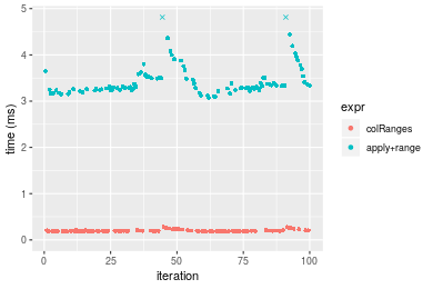
 Table: Benchmarking of colRanges() and rowRanges() on double+100x1000 data (original and transposed). The top panel shows times in milliseconds and the bottom panel shows relative times.
| expr | min | lq | mean | median | uq | max | |
|---|---|---|---|---|---|---|---|
| 1 | colRanges | 179.437 | 189.588 | 201.289 | 194.6985 | 201.708 | 279.644 |
| 2 | rowRanges | 215.885 | 225.069 | 238.594 | 228.6225 | 241.789 | 322.489 |
| expr | min | lq | mean | median | uq | max | |
|---|---|---|---|---|---|---|---|
| 1 | colRanges | 1.000000 | 1.000000 | 1.00000 | 1.000000 | 1.000000 | 1.000000 |
| 2 | rowRanges | 1.203124 | 1.187148 | 1.18533 | 1.174239 | 1.198708 | 1.153213 |
Figure: Benchmarking of colRanges() and rowRanges() on double+100x1000 data (original and transposed). Outliers are displayed as crosses. Times are in milliseconds.
> X <- data[["1000x100"]]
> gc()
          used  (Mb) gc trigger  (Mb) max used  (Mb)
Ncells 3185267 170.2    5709258 305.0  5709258 305.0
Vcells 6149891  47.0   22343563 170.5 56666022 432.4
> colStats <- microbenchmark(colRanges = colRanges(X, na.rm = FALSE), `apply+range` = apply(X, MARGIN = 2L,
+     FUN = range, na.rm = FALSE), unit = "ms")
> X <- t(X)
> gc()
          used  (Mb) gc trigger  (Mb) max used  (Mb)
Ncells 3185258 170.2    5709258 305.0  5709258 305.0
Vcells 6249929  47.7   22343563 170.5 56666022 432.4
> rowStats <- microbenchmark(rowRanges = rowRanges(X, na.rm = FALSE), `apply+range` = apply(X, MARGIN = 1L,
+     FUN = range, na.rm = FALSE), unit = "ms")
Table: Benchmarking of colRanges() and apply+range() on double+1000x100 data. The top panel shows times in milliseconds and the bottom panel shows relative times.
| expr | min | lq | mean | median | uq | max | |
|---|---|---|---|---|---|---|---|
| 1 | colRanges | 0.120533 | 0.122163 | 0.1291061 | 0.123614 | 0.1341775 | 0.164952 |
| 2 | apply+range | 0.981820 | 0.994169 | 1.1872157 | 1.017043 | 1.1041030 | 7.618334 |
| expr | min | lq | mean | median | uq | max | |
|---|---|---|---|---|---|---|---|
| 1 | colRanges | 1.000000 | 1.000000 | 1.000000 | 1.000000 | 1.000000 | 1.00000 |
| 2 | apply+range | 8.145653 | 8.138053 | 9.195659 | 8.227575 | 8.228675 | 46.18516 |
Table: Benchmarking of rowRanges() and apply+range() on double+1000x100 data (transposed). The top panel shows times in milliseconds and the bottom panel shows relative times.
| expr | min | lq | mean | median | uq | max | |
|---|---|---|---|---|---|---|---|
| 1 | rowRanges | 0.174045 | 0.175108 | 0.1864741 | 0.176347 | 0.193471 | 0.311685 |
| 2 | apply+range | 1.011355 | 1.024305 | 1.2291105 | 1.053208 | 1.153560 | 7.734844 |
| expr | min | lq | mean | median | uq | max | |
|---|---|---|---|---|---|---|---|
| 1 | rowRanges | 1.000000 | 1.000000 | 1.00000 | 1.000000 | 1.000000 | 1.00000 |
| 2 | apply+range | 5.810882 | 5.849561 | 6.59132 | 5.972359 | 5.962441 | 24.81622 |
Figure: Benchmarking of colRanges() and apply+range() on double+1000x100 data as well as rowRanges() and apply+range() on the same data transposed. Outliers are displayed as crosses. Times are in milliseconds.

 Table: Benchmarking of colRanges() and rowRanges() on double+1000x100 data (original and transposed). The top panel shows times in milliseconds and the bottom panel shows relative times.
| expr | min | lq | mean | median | uq | max | |
|---|---|---|---|---|---|---|---|
| 1 | colRanges | 120.533 | 122.163 | 129.1061 | 123.614 | 134.1775 | 164.952 |
| 2 | rowRanges | 174.045 | 175.108 | 186.4741 | 176.347 | 193.4710 | 311.685 |
| expr | min | lq | mean | median | uq | max | |
|---|---|---|---|---|---|---|---|
| 1 | colRanges | 1.000000 | 1.000000 | 1.000000 | 1.000000 | 1.000000 | 1.00000 |
| 2 | rowRanges | 1.443961 | 1.433396 | 1.444348 | 1.426594 | 1.441903 | 1.88955 |
Figure: Benchmarking of colRanges() and rowRanges() on double+1000x100 data (original and transposed). Outliers are displayed as crosses. Times are in milliseconds.

R version 3.6.1 Patched (2019-08-27 r77078)
Platform: x86_64-pc-linux-gnu (64-bit)
Running under: Ubuntu 18.04.3 LTS

Matrix products: default
BLAS:   /home/hb/software/R-devel/R-3-6-branch/lib/R/lib/libRblas.so
LAPACK: /home/hb/software/R-devel/R-3-6-branch/lib/R/lib/libRlapack.so

locale:
 [1] LC_CTYPE=en_US.UTF-8       LC_NUMERIC=C
 [3] LC_TIME=en_US.UTF-8        LC_COLLATE=en_US.UTF-8
 [5] LC_MONETARY=en_US.UTF-8    LC_MESSAGES=en_US.UTF-8
 [7] LC_PAPER=en_US.UTF-8       LC_NAME=C
 [9] LC_ADDRESS=C               LC_TELEPHONE=C
[11] LC_MEASUREMENT=en_US.UTF-8 LC_IDENTIFICATION=C

attached base packages:
[1] stats     graphics  grDevices utils     datasets  methods   base

other attached packages:
[1] microbenchmark_1.4-6    matrixStats_0.55.0-9000 ggplot2_3.2.1
[4] knitr_1.24              R.devices_2.16.0        R.utils_2.9.0
[7] R.oo_1.22.0             R.methodsS3_1.7.1       history_0.0.0-9002

loaded via a namespace (and not attached):
 [1] Biobase_2.45.0       bit64_0.9-7          splines_3.6.1
 [4] network_1.15         assertthat_0.2.1     highr_0.8
 [7] stats4_3.6.1         blob_1.2.0           robustbase_0.93-5
[10] pillar_1.4.2         RSQLite_2.1.2        backports_1.1.4
[13] lattice_0.20-38      glue_1.3.1           digest_0.6.20
[16] colorspace_1.4-1     sandwich_2.5-1       Matrix_1.2-17
[19] XML_3.98-1.20        lpSolve_5.6.13.3     pkgconfig_2.0.2
[22] genefilter_1.66.0    purrr_0.3.2          ergm_3.10.4
[25] xtable_1.8-4         mvtnorm_1.0-11       scales_1.0.0
[28] tibble_2.1.3         annotate_1.62.0      IRanges_2.18.2
[31] TH.data_1.0-10       withr_2.1.2          BiocGenerics_0.30.0
[34] lazyeval_0.2.2       mime_0.7             survival_2.44-1.1
[37] magrittr_1.5         crayon_1.3.4         statnet.common_4.3.0
[40] memoise_1.1.0        laeken_0.5.0         R.cache_0.13.0
[43] MASS_7.3-51.4        R.rsp_0.43.1         tools_3.6.1
[46] multcomp_1.4-10      S4Vectors_0.22.1     trust_0.1-7
[49] munsell_0.5.0        AnnotationDbi_1.46.1 compiler_3.6.1
[52] rlang_0.4.0          grid_3.6.1           RCurl_1.95-4.12
[55] cwhmisc_6.6          rappdirs_0.3.1       labeling_0.3
[58] bitops_1.0-6         base64enc_0.1-3      boot_1.3-23
[61] gtable_0.3.0         codetools_0.2-16     DBI_1.0.0
[64] markdown_1.1         R6_2.4.0             zoo_1.8-6
[67] dplyr_0.8.3          bit_1.1-14           zeallot_0.1.0
[70] parallel_3.6.1       Rcpp_1.0.2           vctrs_0.2.0
[73] DEoptimR_1.0-8       tidyselect_0.2.5     xfun_0.9
[76] coda_0.19-3
Total processing time was 25.15 secs.
To reproduce this report, do:
html <- matrixStats:::benchmark('colRanges')Copyright Henrik Bengtsson. Last updated on 2019-09-10 20:51:30 (-0700 UTC). Powered by RSP.
<script> var link = document.createElement('link'); link.rel = 'icon'; link.href = "data:image/png;base64,iVBORw0KGgoAAAANSUhEUgAAACAAAAAgCAMAAABEpIrGAAAA21BMVEUAAAAAAP8AAP8AAP8AAP8AAP8AAP8AAP8AAP8AAP8AAP8AAP8AAP8AAP8AAP8AAP8AAP8AAP8AAP8AAP8AAP8AAP8AAP8AAP8AAP8AAP8AAP8AAP8AAP8AAP8AAP8AAP8AAP8AAP8AAP8AAP8AAP8AAP8AAP8AAP8AAP8AAP8BAf4CAv0DA/wdHeIeHuEfH+AgIN8hId4lJdomJtknJ9g+PsE/P8BAQL9yco10dIt1dYp3d4h4eIeVlWqWlmmXl2iYmGeZmWabm2Tn5xjo6Bfp6Rb39wj4+Af//wA2M9hbAAAASXRSTlMAAQIJCgsMJSYnKD4/QGRlZmhpamtsbautrrCxuru8y8zN5ebn6Pn6+///////////////////////////////////////////LsUNcQAAAS9JREFUOI29k21XgkAQhVcFytdSMqMETU26UVqGmpaiFbL//xc1cAhhwVNf6n5i5z67M2dmYOyfJZUqlVLhkKucG7cgmUZTybDz6g0iDeq51PUr37Ds2cy2/C9NeES5puDjxuUk1xnToZsg8pfA3avHQ3lLIi7iWRrkv/OYtkScxBIMgDee0ALoyxHQBJ68JLCjOtQIMIANF7QG9G9fNnHvisCHBVMKgSJgiz7nE+AoBKrAPA3MgepvgR9TSCasrCKH0eB1wBGBFdCO+nAGjMVGPcQb5bd6mQRegN6+1axOs9nGfYcCtfi4NQosdtH7dB+txFIpXQqN1p9B/asRHToyS0jRgpV7nk4nwcq1BJ+x3Gl/v7S9Wmpp/aGquum7w3ZDyrADFYrl8vHBH+ev9AUASW1dmU4h4wAAAABJRU5ErkJggg==" document.getElementsByTagName('head')[0].appendChild(link); </script>