colRowQuantiles
matrixStats: Benchmark report
This report benchmark the performance of colQuantiles() and rowQuantiles() against alternative methods.
- apply() + quantile()
> rmatrix <- function(nrow, ncol, mode = c("logical", "double", "integer", "index"), range = c(-100,
+     +100), na_prob = 0) {
+     mode <- match.arg(mode)
+     n <- nrow * ncol
+     if (mode == "logical") {
+         x <- sample(c(FALSE, TRUE), size = n, replace = TRUE)
+     }     else if (mode == "index") {
+         x <- seq_len(n)
+         mode <- "integer"
+     }     else {
+         x <- runif(n, min = range[1], max = range[2])
+     }
+     storage.mode(x) <- mode
+     if (na_prob > 0)
+         x[sample(n, size = na_prob * n)] <- NA
+     dim(x) <- c(nrow, ncol)
+     x
+ }
> rmatrices <- function(scale = 10, seed = 1, ...) {
+     set.seed(seed)
+     data <- list()
+     data[[1]] <- rmatrix(nrow = scale * 1, ncol = scale * 1, ...)
+     data[[2]] <- rmatrix(nrow = scale * 10, ncol = scale * 10, ...)
+     data[[3]] <- rmatrix(nrow = scale * 100, ncol = scale * 1, ...)
+     data[[4]] <- t(data[[3]])
+     data[[5]] <- rmatrix(nrow = scale * 10, ncol = scale * 100, ...)
+     data[[6]] <- t(data[[5]])
+     names(data) <- sapply(data, FUN = function(x) paste(dim(x), collapse = "x"))
+     data
+ }
> data <- rmatrices(mode = "double")> X <- data[["10x10"]]
> gc()
used (Mb) gc trigger (Mb) max used (Mb)
Ncells 3179358 169.8 5709258 305.0 5709258 305.0
Vcells 6475075 49.5 22343563 170.5 56666022 432.4
> probs <- seq(from = 0, to = 1, by = 0.25)
> colStats <- microbenchmark(colQuantiles = colQuantiles(X, probs = probs, na.rm = FALSE), `apply+quantile` = apply(X,
+ MARGIN = 2L, FUN = quantile, probs = probs, na.rm = FALSE), unit = "ms")
> X <- t(X)
> gc()
used (Mb) gc trigger (Mb) max used (Mb)
Ncells 3177679 169.8 5709258 305.0 5709258 305.0
Vcells 6470221 49.4 22343563 170.5 56666022 432.4
> rowStats <- microbenchmark(rowQuantiles = rowQuantiles(X, probs = probs, na.rm = FALSE), `apply+quantile` = apply(X,
+ MARGIN = 1L, FUN = quantile, probs = probs, na.rm = FALSE), unit = "ms")Table: Benchmarking of colQuantiles() and apply+quantile() on 10x10 data. The top panel shows times in milliseconds and the bottom panel shows relative times.
| expr | min | lq | mean | median | uq | max | |
|---|---|---|---|---|---|---|---|
| 1 | colQuantiles | 0.204771 | 0.2105605 | 0.2178498 | 0.215639 | 0.2237735 | 0.277387 |
| 2 | apply+quantile | 0.749683 | 0.7618105 | 0.7855426 | 0.778345 | 0.8060455 | 1.075560 |
| expr | min | lq | mean | median | uq | max | |
|---|---|---|---|---|---|---|---|
| 1 | colQuantiles | 1.00000 | 1.000000 | 1.000000 | 1.000000 | 1.00000 | 1.000000 |
| 2 | apply+quantile | 3.66108 | 3.618012 | 3.605891 | 3.609482 | 3.60206 | 3.877471 |
Table: Benchmarking of rowQuantiles() and apply+quantile() on 10x10 data (transposed). The top panel shows times in milliseconds and the bottom panel shows relative times.
| expr | min | lq | mean | median | uq | max | |
|---|---|---|---|---|---|---|---|
| 1 | rowQuantiles | 0.206766 | 0.2157140 | 0.2280534 | 0.224474 | 0.2295620 | 0.284570 |
| 2 | apply+quantile | 0.752545 | 0.7676515 | 0.8118481 | 0.801476 | 0.8111235 | 1.064999 |
| expr | min | lq | mean | median | uq | max | |
|---|---|---|---|---|---|---|---|
| 1 | rowQuantiles | 1.000000 | 1.000000 | 1.000000 | 1.000000 | 1.000000 | 1.000000 |
| 2 | apply+quantile | 3.639597 | 3.558654 | 3.559904 | 3.570463 | 3.533353 | 3.742485 |
Figure: Benchmarking of colQuantiles() and apply+quantile() on 10x10 data as well as rowQuantiles() and apply+quantile() on the same data transposed. Outliers are displayed as crosses. Times are in milliseconds.

 Table: Benchmarking of colQuantiles() and rowQuantiles() on 10x10 data (original and transposed). The top panel shows times in milliseconds and the bottom panel shows relative times.
| expr | min | lq | mean | median | uq | max | |
|---|---|---|---|---|---|---|---|
| 1 | colQuantiles | 204.771 | 210.5605 | 217.8498 | 215.639 | 223.7735 | 277.387 |
| 2 | rowQuantiles | 206.766 | 215.7140 | 228.0534 | 224.474 | 229.5620 | 284.570 |
| expr | min | lq | mean | median | uq | max | |
|---|---|---|---|---|---|---|---|
| 1 | colQuantiles | 1.000000 | 1.000000 | 1.000000 | 1.000000 | 1.000000 | 1.000000 |
| 2 | rowQuantiles | 1.009743 | 1.024475 | 1.046838 | 1.040971 | 1.025868 | 1.025895 |
Figure: Benchmarking of colQuantiles() and rowQuantiles() on 10x10 data (original and transposed). Outliers are displayed as crosses. Times are in milliseconds.

> X <- data[["100x100"]]
> gc()
          used  (Mb) gc trigger  (Mb) max used  (Mb)
Ncells 3176235 169.7    5709258 305.0  5709258 305.0
Vcells 6086658  46.5   22343563 170.5 56666022 432.4
> probs <- seq(from = 0, to = 1, by = 0.25)
> colStats <- microbenchmark(colQuantiles = colQuantiles(X, probs = probs, na.rm = FALSE), `apply+quantile` = apply(X,
+     MARGIN = 2L, FUN = quantile, probs = probs, na.rm = FALSE), unit = "ms")
> X <- t(X)
> gc()
          used  (Mb) gc trigger  (Mb) max used  (Mb)
Ncells 3176226 169.7    5709258 305.0  5709258 305.0
Vcells 6096696  46.6   22343563 170.5 56666022 432.4
> rowStats <- microbenchmark(rowQuantiles = rowQuantiles(X, probs = probs, na.rm = FALSE), `apply+quantile` = apply(X,
+     MARGIN = 1L, FUN = quantile, probs = probs, na.rm = FALSE), unit = "ms")
Table: Benchmarking of colQuantiles() and apply+quantile() on 100x100 data. The top panel shows times in milliseconds and the bottom panel shows relative times.
| expr | min | lq | mean | median | uq | max | |
|---|---|---|---|---|---|---|---|
| 1 | colQuantiles | 1.667526 | 1.717488 | 1.805961 | 1.755473 | 1.828817 | 2.532032 |
| 2 | apply+quantile | 7.725793 | 7.869764 | 8.623150 | 7.984455 | 8.368327 | 24.770606 |
| expr | min | lq | mean | median | uq | max | |
|---|---|---|---|---|---|---|---|
| 1 | colQuantiles | 1.000000 | 1.000000 | 1.000000 | 1.000000 | 1.000000 | 1.000000 |
| 2 | apply+quantile | 4.633087 | 4.582135 | 4.774825 | 4.548321 | 4.575813 | 9.782896 |
Table: Benchmarking of rowQuantiles() and apply+quantile() on 100x100 data (transposed). The top panel shows times in milliseconds and the bottom panel shows relative times.
| expr | min | lq | mean | median | uq | max | |
|---|---|---|---|---|---|---|---|
| 1 | rowQuantiles | 1.703577 | 1.743685 | 1.818584 | 1.790552 | 1.831886 | 2.262452 |
| 2 | apply+quantile | 7.699512 | 7.821835 | 8.453948 | 7.928989 | 8.204308 | 17.136500 |
| expr | min | lq | mean | median | uq | max | |
|---|---|---|---|---|---|---|---|
| 1 | rowQuantiles | 1.000000 | 1.000000 | 1.000000 | 1.000000 | 1.000000 | 1.000000 |
| 2 | apply+quantile | 4.519615 | 4.485806 | 4.648644 | 4.428238 | 4.478612 | 7.574304 |
Figure: Benchmarking of colQuantiles() and apply+quantile() on 100x100 data as well as rowQuantiles() and apply+quantile() on the same data transposed. Outliers are displayed as crosses. Times are in milliseconds.

 Table: Benchmarking of colQuantiles() and rowQuantiles() on 100x100 data (original and transposed). The top panel shows times in milliseconds and the bottom panel shows relative times.
| expr | min | lq | mean | median | uq | max | |
|---|---|---|---|---|---|---|---|
| 1 | colQuantiles | 1.667526 | 1.717488 | 1.805961 | 1.755473 | 1.828817 | 2.532032 |
| 2 | rowQuantiles | 1.703577 | 1.743685 | 1.818584 | 1.790552 | 1.831886 | 2.262452 |
| expr | min | lq | mean | median | uq | max | |
|---|---|---|---|---|---|---|---|
| 1 | colQuantiles | 1.000000 | 1.000000 | 1.000000 | 1.000000 | 1.000000 | 1.0000000 |
| 2 | rowQuantiles | 1.021619 | 1.015253 | 1.006989 | 1.019982 | 1.001678 | 0.8935322 |
Figure: Benchmarking of colQuantiles() and rowQuantiles() on 100x100 data (original and transposed). Outliers are displayed as crosses. Times are in milliseconds.

> X <- data[["1000x10"]]
> gc()
          used  (Mb) gc trigger  (Mb) max used  (Mb)
Ncells 3176965 169.7    5709258 305.0  5709258 305.0
Vcells 6090169  46.5   22343563 170.5 56666022 432.4
> probs <- seq(from = 0, to = 1, by = 0.25)
> colStats <- microbenchmark(colQuantiles = colQuantiles(X, probs = probs, na.rm = FALSE), `apply+quantile` = apply(X,
+     MARGIN = 2L, FUN = quantile, probs = probs, na.rm = FALSE), unit = "ms")
> X <- t(X)
> gc()
          used  (Mb) gc trigger  (Mb) max used  (Mb)
Ncells 3176956 169.7    5709258 305.0  5709258 305.0
Vcells 6100207  46.6   22343563 170.5 56666022 432.4
> rowStats <- microbenchmark(rowQuantiles = rowQuantiles(X, probs = probs, na.rm = FALSE), `apply+quantile` = apply(X,
+     MARGIN = 1L, FUN = quantile, probs = probs, na.rm = FALSE), unit = "ms")
Table: Benchmarking of colQuantiles() and apply+quantile() on 1000x10 data. The top panel shows times in milliseconds and the bottom panel shows relative times.
| expr | min | lq | mean | median | uq | max | |
|---|---|---|---|---|---|---|---|
| 1 | colQuantiles | 0.569989 | 0.5843265 | 0.5998415 | 0.5927725 | 0.598683 | 0.944226 |
| 2 | apply+quantile | 1.240029 | 1.2566525 | 1.2884913 | 1.2720650 | 1.284201 | 1.816026 |
| expr | min | lq | mean | median | uq | max | |
|---|---|---|---|---|---|---|---|
| 1 | colQuantiles | 1.000000 | 1.0000 | 1.000000 | 1.000000 | 1.000000 | 1.000000 |
| 2 | apply+quantile | 2.175531 | 2.1506 | 2.148053 | 2.145958 | 2.145043 | 1.923296 |
Table: Benchmarking of rowQuantiles() and apply+quantile() on 1000x10 data (transposed). The top panel shows times in milliseconds and the bottom panel shows relative times.
| expr | min | lq | mean | median | uq | max | |
|---|---|---|---|---|---|---|---|
| 1 | rowQuantiles | 0.579148 | 0.591894 | 0.6044141 | 0.6020005 | 0.607459 | 0.844155 |
| 2 | apply+quantile | 1.189937 | 1.215024 | 1.2409754 | 1.2348835 | 1.244353 | 1.698761 |
| expr | min | lq | mean | median | uq | max | |
|---|---|---|---|---|---|---|---|
| 1 | rowQuantiles | 1.000000 | 1.000000 | 1.000000 | 1.0000 | 1.000000 | 1.00000 |
| 2 | apply+quantile | 2.054634 | 2.052772 | 2.053187 | 2.0513 | 2.048456 | 2.01238 |
Figure: Benchmarking of colQuantiles() and apply+quantile() on 1000x10 data as well as rowQuantiles() and apply+quantile() on the same data transposed. Outliers are displayed as crosses. Times are in milliseconds.

 Table: Benchmarking of colQuantiles() and rowQuantiles() on 1000x10 data (original and transposed). The top panel shows times in milliseconds and the bottom panel shows relative times.
| expr | min | lq | mean | median | uq | max | |
|---|---|---|---|---|---|---|---|
| 1 | colQuantiles | 569.989 | 584.3265 | 599.8415 | 592.7725 | 598.683 | 944.226 |
| 2 | rowQuantiles | 579.148 | 591.8940 | 604.4141 | 602.0005 | 607.459 | 844.155 |
| expr | min | lq | mean | median | uq | max | |
|---|---|---|---|---|---|---|---|
| 1 | colQuantiles | 1.000000 | 1.000000 | 1.000000 | 1.000000 | 1.000000 | 1.000000 |
| 2 | rowQuantiles | 1.016069 | 1.012951 | 1.007623 | 1.015567 | 1.014659 | 0.894018 |
Figure: Benchmarking of colQuantiles() and rowQuantiles() on 1000x10 data (original and transposed). Outliers are displayed as crosses. Times are in milliseconds.

> X <- data[["10x1000"]]
> gc()
          used  (Mb) gc trigger  (Mb) max used  (Mb)
Ncells 3177153 169.7    5709258 305.0  5709258 305.0
Vcells 6090883  46.5   22343563 170.5 56666022 432.4
> probs <- seq(from = 0, to = 1, by = 0.25)
> colStats <- microbenchmark(colQuantiles = colQuantiles(X, probs = probs, na.rm = FALSE), `apply+quantile` = apply(X,
+     MARGIN = 2L, FUN = quantile, probs = probs, na.rm = FALSE), unit = "ms")
> X <- t(X)
> gc()
          used  (Mb) gc trigger  (Mb) max used  (Mb)
Ncells 3177144 169.7    5709258 305.0  5709258 305.0
Vcells 6100921  46.6   22343563 170.5 56666022 432.4
> rowStats <- microbenchmark(rowQuantiles = rowQuantiles(X, probs = probs, na.rm = FALSE), `apply+quantile` = apply(X,
+     MARGIN = 1L, FUN = quantile, probs = probs, na.rm = FALSE), unit = "ms")
Table: Benchmarking of colQuantiles() and apply+quantile() on 10x1000 data. The top panel shows times in milliseconds and the bottom panel shows relative times.
| expr | min | lq | mean | median | uq | max | |
|---|---|---|---|---|---|---|---|
| 1 | colQuantiles | 11.71571 | 12.18752 | 13.55159 | 12.58262 | 13.51043 | 25.37621 |
| 2 | apply+quantile | 71.34555 | 73.34382 | 79.28271 | 75.91291 | 86.14064 | 111.41644 |
| expr | min | lq | mean | median | uq | max | |
|---|---|---|---|---|---|---|---|
| 1 | colQuantiles | 1.000000 | 1.000000 | 1.000000 | 1.000000 | 1.000000 | 1.000000 |
| 2 | apply+quantile | 6.089731 | 6.017944 | 5.850437 | 6.033157 | 6.375863 | 4.390586 |
Table: Benchmarking of rowQuantiles() and apply+quantile() on 10x1000 data (transposed). The top panel shows times in milliseconds and the bottom panel shows relative times.
| expr | min | lq | mean | median | uq | max | |
|---|---|---|---|---|---|---|---|
| 1 | rowQuantiles | 11.76357 | 12.18355 | 15.75459 | 12.62987 | 12.87938 | 266.1704 |
| 2 | apply+quantile | 70.98810 | 72.54362 | 77.77507 | 74.25125 | 84.08314 | 110.3797 |
| expr | min | lq | mean | median | uq | max | |
|---|---|---|---|---|---|---|---|
| 1 | rowQuantiles | 1.000000 | 1.000000 | 1.000000 | 1.00000 | 1.00000 | 1.0000000 |
| 2 | apply+quantile | 6.034569 | 5.954227 | 4.936662 | 5.87902 | 6.52851 | 0.4146957 |
Figure: Benchmarking of colQuantiles() and apply+quantile() on 10x1000 data as well as rowQuantiles() and apply+quantile() on the same data transposed. Outliers are displayed as crosses. Times are in milliseconds.
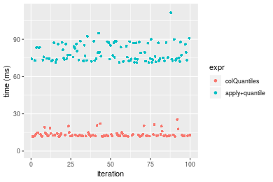
 Table: Benchmarking of colQuantiles() and rowQuantiles() on 10x1000 data (original and transposed). The top panel shows times in milliseconds and the bottom panel shows relative times.
| expr | min | lq | mean | median | uq | max | |
|---|---|---|---|---|---|---|---|
| 1 | colQuantiles | 11.71571 | 12.18752 | 13.55159 | 12.58262 | 13.51043 | 25.37621 |
| 2 | rowQuantiles | 11.76357 | 12.18355 | 15.75459 | 12.62987 | 12.87938 | 266.17038 |
| expr | min | lq | mean | median | uq | max | |
|---|---|---|---|---|---|---|---|
| 1 | colQuantiles | 1.000000 | 1.0000000 | 1.000000 | 1.000000 | 1.0000000 | 1.00000 |
| 2 | rowQuantiles | 1.004085 | 0.9996741 | 1.162564 | 1.003755 | 0.9532915 | 10.48897 |
Figure: Benchmarking of colQuantiles() and rowQuantiles() on 10x1000 data (original and transposed). Outliers are displayed as crosses. Times are in milliseconds.

> X <- data[["100x1000"]]
> gc()
          used  (Mb) gc trigger  (Mb) max used  (Mb)
Ncells 3177337 169.7    5709258 305.0  5709258 305.0
Vcells 6091379  46.5   22343563 170.5 56666022 432.4
> probs <- seq(from = 0, to = 1, by = 0.25)
> colStats <- microbenchmark(colQuantiles = colQuantiles(X, probs = probs, na.rm = FALSE), `apply+quantile` = apply(X,
+     MARGIN = 2L, FUN = quantile, probs = probs, na.rm = FALSE), unit = "ms")
> X <- t(X)
> gc()
          used  (Mb) gc trigger  (Mb) max used  (Mb)
Ncells 3177328 169.7    5709258 305.0  5709258 305.0
Vcells 6191417  47.3   22343563 170.5 56666022 432.4
> rowStats <- microbenchmark(rowQuantiles = rowQuantiles(X, probs = probs, na.rm = FALSE), `apply+quantile` = apply(X,
+     MARGIN = 1L, FUN = quantile, probs = probs, na.rm = FALSE), unit = "ms")
Table: Benchmarking of colQuantiles() and apply+quantile() on 100x1000 data. The top panel shows times in milliseconds and the bottom panel shows relative times.
| expr | min | lq | mean | median | uq | max | |
|---|---|---|---|---|---|---|---|
| 1 | colQuantiles | 15.94949 | 16.39826 | 18.22907 | 17.03291 | 17.93682 | 37.48265 |
| 2 | apply+quantile | 78.03791 | 80.35847 | 86.19026 | 81.81766 | 91.94407 | 122.29199 |
| expr | min | lq | mean | median | uq | max | |
|---|---|---|---|---|---|---|---|
| 1 | colQuantiles | 1.000000 | 1.000000 | 1.000000 | 1.000000 | 1.000000 | 1.000000 |
| 2 | apply+quantile | 4.892816 | 4.900427 | 4.728176 | 4.803505 | 5.125998 | 3.262629 |
Table: Benchmarking of rowQuantiles() and apply+quantile() on 100x1000 data (transposed). The top panel shows times in milliseconds and the bottom panel shows relative times.
| expr | min | lq | mean | median | uq | max | |
|---|---|---|---|---|---|---|---|
| 1 | rowQuantiles | 16.22328 | 16.82461 | 19.30184 | 17.49396 | 19.63542 | 46.58731 |
| 2 | apply+quantile | 77.73885 | 80.14350 | 88.41864 | 82.86826 | 94.35297 | 134.76324 |
| expr | min | lq | mean | median | uq | max | |
|---|---|---|---|---|---|---|---|
| 1 | rowQuantiles | 1.000000 | 1.000000 | 1.000000 | 1.000000 | 1.000000 | 1.000000 |
| 2 | apply+quantile | 4.791808 | 4.763469 | 4.580839 | 4.736965 | 4.805243 | 2.892703 |
Figure: Benchmarking of colQuantiles() and apply+quantile() on 100x1000 data as well as rowQuantiles() and apply+quantile() on the same data transposed. Outliers are displayed as crosses. Times are in milliseconds.

 Table: Benchmarking of colQuantiles() and rowQuantiles() on 100x1000 data (original and transposed). The top panel shows times in milliseconds and the bottom panel shows relative times.
| expr | min | lq | mean | median | uq | max | |
|---|---|---|---|---|---|---|---|
| 1 | colQuantiles | 15.94949 | 16.39826 | 18.22907 | 17.03291 | 17.93682 | 37.48265 |
| 2 | rowQuantiles | 16.22328 | 16.82461 | 19.30184 | 17.49396 | 19.63542 | 46.58731 |
| expr | min | lq | mean | median | uq | max | |
|---|---|---|---|---|---|---|---|
| 1 | colQuantiles | 1.000000 | 1.000 | 1.000000 | 1.000000 | 1.000000 | 1.000000 |
| 2 | rowQuantiles | 1.017166 | 1.026 | 1.058849 | 1.027068 | 1.094699 | 1.242903 |
Figure: Benchmarking of colQuantiles() and rowQuantiles() on 100x1000 data (original and transposed). Outliers are displayed as crosses. Times are in milliseconds.

> X <- data[["1000x100"]]
> gc()
          used  (Mb) gc trigger  (Mb) max used  (Mb)
Ncells 3177529 169.7    5709258 305.0  5709258 305.0
Vcells 6091993  46.5   22343563 170.5 56666022 432.4
> probs <- seq(from = 0, to = 1, by = 0.25)
> colStats <- microbenchmark(colQuantiles = colQuantiles(X, probs = probs, na.rm = FALSE), `apply+quantile` = apply(X,
+     MARGIN = 2L, FUN = quantile, probs = probs, na.rm = FALSE), unit = "ms")
> X <- t(X)
> gc()
          used  (Mb) gc trigger  (Mb) max used  (Mb)
Ncells 3177520 169.7    5709258 305.0  5709258 305.0
Vcells 6192031  47.3   22343563 170.5 56666022 432.4
> rowStats <- microbenchmark(rowQuantiles = rowQuantiles(X, probs = probs, na.rm = FALSE), `apply+quantile` = apply(X,
+     MARGIN = 1L, FUN = quantile, probs = probs, na.rm = FALSE), unit = "ms")
Table: Benchmarking of colQuantiles() and apply+quantile() on 1000x100 data. The top panel shows times in milliseconds and the bottom panel shows relative times.
| expr | min | lq | mean | median | uq | max | |
|---|---|---|---|---|---|---|---|
| 1 | colQuantiles | 4.794218 | 4.948212 | 5.233887 | 4.99597 | 5.095167 | 13.85089 |
| 2 | apply+quantile | 11.677002 | 11.793934 | 12.435548 | 11.91788 | 12.195339 | 22.84092 |
| expr | min | lq | mean | median | uq | max | |
|---|---|---|---|---|---|---|---|
| 1 | colQuantiles | 1.000000 | 1.000000 | 1.000000 | 1.000000 | 1.000000 | 1.000000 |
| 2 | apply+quantile | 2.435643 | 2.383474 | 2.375968 | 2.385499 | 2.393511 | 1.649059 |
Table: Benchmarking of rowQuantiles() and apply+quantile() on 1000x100 data (transposed). The top panel shows times in milliseconds and the bottom panel shows relative times.
| expr | min | lq | mean | median | uq | max | |
|---|---|---|---|---|---|---|---|
| 1 | rowQuantiles | 5.167341 | 5.26751 | 5.53447 | 5.32830 | 5.388846 | 13.79203 |
| 2 | apply+quantile | 11.684250 | 11.81924 | 12.29935 | 11.91869 | 12.181646 | 22.81130 |
| expr | min | lq | mean | median | uq | max | |
|---|---|---|---|---|---|---|---|
| 1 | rowQuantiles | 1.000000 | 1.0000 | 1.000000 | 1.000000 | 1.00000 | 1.000000 |
| 2 | apply+quantile | 2.261173 | 2.2438 | 2.222318 | 2.236865 | 2.26053 | 1.653948 |
Figure: Benchmarking of colQuantiles() and apply+quantile() on 1000x100 data as well as rowQuantiles() and apply+quantile() on the same data transposed. Outliers are displayed as crosses. Times are in milliseconds.

 Table: Benchmarking of colQuantiles() and rowQuantiles() on 1000x100 data (original and transposed). The top panel shows times in milliseconds and the bottom panel shows relative times.
| expr | min | lq | mean | median | uq | max | |
|---|---|---|---|---|---|---|---|
| 1 | colQuantiles | 4.794218 | 4.948212 | 5.233887 | 4.99597 | 5.095167 | 13.85089 |
| 2 | rowQuantiles | 5.167341 | 5.267510 | 5.534470 | 5.32830 | 5.388846 | 13.79203 |
| expr | min | lq | mean | median | uq | max | |
|---|---|---|---|---|---|---|---|
| 1 | colQuantiles | 1.000000 | 1.000000 | 1.00000 | 1.00000 | 1.000000 | 1.0000000 |
| 2 | rowQuantiles | 1.077828 | 1.064528 | 1.05743 | 1.06652 | 1.057639 | 0.9957505 |
Figure: Benchmarking of colQuantiles() and rowQuantiles() on 1000x100 data (original and transposed). Outliers are displayed as crosses. Times are in milliseconds.

R version 3.6.1 Patched (2019-08-27 r77078)
Platform: x86_64-pc-linux-gnu (64-bit)
Running under: Ubuntu 18.04.3 LTS

Matrix products: default
BLAS:   /home/hb/software/R-devel/R-3-6-branch/lib/R/lib/libRblas.so
LAPACK: /home/hb/software/R-devel/R-3-6-branch/lib/R/lib/libRlapack.so

locale:
 [1] LC_CTYPE=en_US.UTF-8       LC_NUMERIC=C
 [3] LC_TIME=en_US.UTF-8        LC_COLLATE=en_US.UTF-8
 [5] LC_MONETARY=en_US.UTF-8    LC_MESSAGES=en_US.UTF-8
 [7] LC_PAPER=en_US.UTF-8       LC_NAME=C
 [9] LC_ADDRESS=C               LC_TELEPHONE=C
[11] LC_MEASUREMENT=en_US.UTF-8 LC_IDENTIFICATION=C

attached base packages:
[1] stats     graphics  grDevices utils     datasets  methods   base

other attached packages:
[1] microbenchmark_1.4-6    matrixStats_0.55.0-9000 ggplot2_3.2.1
[4] knitr_1.24              R.devices_2.16.0        R.utils_2.9.0
[7] R.oo_1.22.0             R.methodsS3_1.7.1       history_0.0.0-9002

loaded via a namespace (and not attached):
 [1] Biobase_2.45.0       bit64_0.9-7          splines_3.6.1
 [4] network_1.15         assertthat_0.2.1     highr_0.8
 [7] stats4_3.6.1         blob_1.2.0           robustbase_0.93-5
[10] pillar_1.4.2         RSQLite_2.1.2        backports_1.1.4
[13] lattice_0.20-38      glue_1.3.1           digest_0.6.20
[16] colorspace_1.4-1     sandwich_2.5-1       Matrix_1.2-17
[19] XML_3.98-1.20        lpSolve_5.6.13.3     pkgconfig_2.0.2
[22] genefilter_1.66.0    purrr_0.3.2          ergm_3.10.4
[25] xtable_1.8-4         mvtnorm_1.0-11       scales_1.0.0
[28] tibble_2.1.3         annotate_1.62.0      IRanges_2.18.2
[31] TH.data_1.0-10       withr_2.1.2          BiocGenerics_0.30.0
[34] lazyeval_0.2.2       mime_0.7             survival_2.44-1.1
[37] magrittr_1.5         crayon_1.3.4         statnet.common_4.3.0
[40] memoise_1.1.0        laeken_0.5.0         R.cache_0.13.0
[43] MASS_7.3-51.4        R.rsp_0.43.1         tools_3.6.1
[46] multcomp_1.4-10      S4Vectors_0.22.1     trust_0.1-7
[49] munsell_0.5.0        AnnotationDbi_1.46.1 compiler_3.6.1
[52] rlang_0.4.0          grid_3.6.1           RCurl_1.95-4.12
[55] cwhmisc_6.6          rappdirs_0.3.1       labeling_0.3
[58] bitops_1.0-6         base64enc_0.1-3      boot_1.3-23
[61] gtable_0.3.0         codetools_0.2-16     DBI_1.0.0
[64] markdown_1.1         R6_2.4.0             zoo_1.8-6
[67] dplyr_0.8.3          bit_1.1-14           zeallot_0.1.0
[70] parallel_3.6.1       Rcpp_1.0.2           vctrs_0.2.0
[73] DEoptimR_1.0-8       tidyselect_0.2.5     xfun_0.9
[76] coda_0.19-3
Total processing time was 57.27 secs.
To reproduce this report, do:
html <- matrixStats:::benchmark('colQuantiles')Copyright Henrik Bengtsson. Last updated on 2019-09-10 20:50:39 (-0700 UTC). Powered by RSP.
<script> var link = document.createElement('link'); link.rel = 'icon'; link.href = "data:image/png;base64,iVBORw0KGgoAAAANSUhEUgAAACAAAAAgCAMAAABEpIrGAAAA21BMVEUAAAAAAP8AAP8AAP8AAP8AAP8AAP8AAP8AAP8AAP8AAP8AAP8AAP8AAP8AAP8AAP8AAP8AAP8AAP8AAP8AAP8AAP8AAP8AAP8AAP8AAP8AAP8AAP8AAP8AAP8AAP8AAP8AAP8AAP8AAP8AAP8AAP8AAP8AAP8AAP8AAP8AAP8BAf4CAv0DA/wdHeIeHuEfH+AgIN8hId4lJdomJtknJ9g+PsE/P8BAQL9yco10dIt1dYp3d4h4eIeVlWqWlmmXl2iYmGeZmWabm2Tn5xjo6Bfp6Rb39wj4+Af//wA2M9hbAAAASXRSTlMAAQIJCgsMJSYnKD4/QGRlZmhpamtsbautrrCxuru8y8zN5ebn6Pn6+///////////////////////////////////////////LsUNcQAAAS9JREFUOI29k21XgkAQhVcFytdSMqMETU26UVqGmpaiFbL//xc1cAhhwVNf6n5i5z67M2dmYOyfJZUqlVLhkKucG7cgmUZTybDz6g0iDeq51PUr37Ds2cy2/C9NeES5puDjxuUk1xnToZsg8pfA3avHQ3lLIi7iWRrkv/OYtkScxBIMgDee0ALoyxHQBJ68JLCjOtQIMIANF7QG9G9fNnHvisCHBVMKgSJgiz7nE+AoBKrAPA3MgepvgR9TSCasrCKH0eB1wBGBFdCO+nAGjMVGPcQb5bd6mQRegN6+1axOs9nGfYcCtfi4NQosdtH7dB+txFIpXQqN1p9B/asRHToyS0jRgpV7nk4nwcq1BJ+x3Gl/v7S9Wmpp/aGquum7w3ZDyrADFYrl8vHBH+ev9AUASW1dmU4h4wAAAABJRU5ErkJggg==" document.getElementsByTagName('head')[0].appendChild(link); </script>