colRowQuantiles_subset
matrixStats: Benchmark report
This report benchmark the performance of colQuantiles() and rowQuantiles() on subsetted computation.
> rmatrix <- function(nrow, ncol, mode = c("logical", "double", "integer", "index"), range = c(-100,
+     +100), na_prob = 0) {
+     mode <- match.arg(mode)
+     n <- nrow * ncol
+     if (mode == "logical") {
+         x <- sample(c(FALSE, TRUE), size = n, replace = TRUE)
+     }     else if (mode == "index") {
+         x <- seq_len(n)
+         mode <- "integer"
+     }     else {
+         x <- runif(n, min = range[1], max = range[2])
+     }
+     storage.mode(x) <- mode
+     if (na_prob > 0)
+         x[sample(n, size = na_prob * n)] <- NA
+     dim(x) <- c(nrow, ncol)
+     x
+ }
> rmatrices <- function(scale = 10, seed = 1, ...) {
+     set.seed(seed)
+     data <- list()
+     data[[1]] <- rmatrix(nrow = scale * 1, ncol = scale * 1, ...)
+     data[[2]] <- rmatrix(nrow = scale * 10, ncol = scale * 10, ...)
+     data[[3]] <- rmatrix(nrow = scale * 100, ncol = scale * 1, ...)
+     data[[4]] <- t(data[[3]])
+     data[[5]] <- rmatrix(nrow = scale * 10, ncol = scale * 100, ...)
+     data[[6]] <- t(data[[5]])
+     names(data) <- sapply(data, FUN = function(x) paste(dim(x), collapse = "x"))
+     data
+ }
> data <- rmatrices(mode = "double")> X <- data[["10x10"]]
> rows <- sample.int(nrow(X), size = nrow(X) * 0.7)
> cols <- sample.int(ncol(X), size = ncol(X) * 0.7)
> X_S <- X[rows, cols]
> gc()
used (Mb) gc trigger (Mb) max used (Mb)
Ncells 3175014 169.6 5709258 305.0 5709258 305.0
Vcells 6396981 48.9 22343563 170.5 56666022 432.4
> probs <- seq(from = 0, to = 1, by = 0.25)
> colStats <- microbenchmark(colQuantiles_X_S = colQuantiles(X_S, probs = probs, na.rm = FALSE), `colQuantiles(X, rows, cols)` = colQuantiles(X,
+ rows = rows, cols = cols, probs = probs, na.rm = FALSE), `colQuantiles(X[rows, cols])` = colQuantiles(X[rows,
+ cols], probs = probs, na.rm = FALSE), unit = "ms")
> X <- t(X)
> X_S <- t(X_S)
> gc()
used (Mb) gc trigger (Mb) max used (Mb)
Ncells 3174277 169.6 5709258 305.0 5709258 305.0
Vcells 6394473 48.8 22343563 170.5 56666022 432.4
> rowStats <- microbenchmark(rowQuantiles_X_S = rowQuantiles(X_S, probs = probs, na.rm = FALSE), `rowQuantiles(X, cols, rows)` = rowQuantiles(X,
+ rows = cols, cols = rows, probs = probs, na.rm = FALSE), `rowQuantiles(X[cols, rows])` = rowQuantiles(X[cols,
+ rows], probs = probs, na.rm = FALSE), unit = "ms")Table: Benchmarking of colQuantiles_X_S(), colQuantiles(X, rows, cols)() and colQuantiles(X[rows, cols])() on 10x10 data. The top panel shows times in milliseconds and the bottom panel shows relative times.
| expr | min | lq | mean | median | uq | max | |
|---|---|---|---|---|---|---|---|
| 1 | colQuantiles_X_S | 0.159063 | 0.1612190 | 0.1679418 | 0.1621265 | 0.1632945 | 0.678460 |
| 3 | colQuantiles(X[rows, cols]) | 0.160790 | 0.1627480 | 0.1645033 | 0.1638575 | 0.1652030 | 0.179393 |
| 2 | colQuantiles(X, rows, cols) | 0.160587 | 0.1633335 | 0.1651102 | 0.1643465 | 0.1662740 | 0.179827 |
| expr | min | lq | mean | median | uq | max | |
|---|---|---|---|---|---|---|---|
| 1 | colQuantiles_X_S | 1.000000 | 1.000000 | 1.0000000 | 1.000000 | 1.000000 | 1.0000000 |
| 3 | colQuantiles(X[rows, cols]) | 1.010857 | 1.009484 | 0.9795252 | 1.010677 | 1.011688 | 0.2644121 |
| 2 | colQuantiles(X, rows, cols) | 1.009581 | 1.013116 | 0.9831392 | 1.013693 | 1.018246 | 0.2650517 |
Table: Benchmarking of rowQuantiles_X_S(), rowQuantiles(X, cols, rows)() and rowQuantiles(X[cols, rows])() on 10x10 data (transposed). The top panel shows times in milliseconds and the bottom panel shows relative times.
| expr | min | lq | mean | median | uq | max | |
|---|---|---|---|---|---|---|---|
| 1 | rowQuantiles_X_S | 0.160542 | 0.1631545 | 0.1649297 | 0.1641865 | 0.1662660 | 0.178008 |
| 3 | rowQuantiles(X[cols, rows]) | 0.162827 | 0.1643365 | 0.1673207 | 0.1654305 | 0.1669935 | 0.282405 |
| 2 | rowQuantiles(X, cols, rows) | 0.162740 | 0.1647915 | 0.1721287 | 0.1658600 | 0.1675075 | 0.673119 |
| expr | min | lq | mean | median | uq | max | |
|---|---|---|---|---|---|---|---|
| 1 | rowQuantiles_X_S | 1.000000 | 1.000000 | 1.000000 | 1.000000 | 1.000000 | 1.000000 |
| 3 | rowQuantiles(X[cols, rows]) | 1.014233 | 1.007245 | 1.014497 | 1.007577 | 1.004376 | 1.586474 |
| 2 | rowQuantiles(X, cols, rows) | 1.013691 | 1.010033 | 1.043648 | 1.010193 | 1.007467 | 3.781398 |
Figure: Benchmarking of colQuantiles_X_S(), colQuantiles(X, rows, cols)() and colQuantiles(X[rows, cols])() on 10x10 data as well as rowQuantiles_X_S(), rowQuantiles(X, cols, rows)() and rowQuantiles(X[cols, rows])() on the same data transposed. Outliers are displayed as crosses. Times are in milliseconds.

 Table: Benchmarking of colQuantiles_X_S() and rowQuantiles_X_S() on 10x10 data (original and transposed). The top panel shows times in milliseconds and the bottom panel shows relative times.
| expr | min | lq | mean | median | uq | max | |
|---|---|---|---|---|---|---|---|
| 1 | colQuantiles_X_S | 159.063 | 161.2190 | 167.9418 | 162.1265 | 163.2945 | 678.460 |
| 2 | rowQuantiles_X_S | 160.542 | 163.1545 | 164.9298 | 164.1865 | 166.2660 | 178.008 |
| expr | min | lq | mean | median | uq | max | |
|---|---|---|---|---|---|---|---|
| 1 | colQuantiles_X_S | 1.000000 | 1.000000 | 1.0000000 | 1.000000 | 1.000000 | 1.0000000 |
| 2 | rowQuantiles_X_S | 1.009298 | 1.012005 | 0.9820646 | 1.012706 | 1.018197 | 0.2623707 |
Figure: Benchmarking of colQuantiles_X_S() and rowQuantiles_X_S() on 10x10 data (original and transposed). Outliers are displayed as crosses. Times are in milliseconds.

> X <- data[["100x100"]]
> rows <- sample.int(nrow(X), size = nrow(X) * 0.7)
> cols <- sample.int(ncol(X), size = ncol(X) * 0.7)
> X_S <- X[rows, cols]
> gc()
          used  (Mb) gc trigger  (Mb) max used  (Mb)
Ncells 3173822 169.6    5709258 305.0  5709258 305.0
Vcells 6067332  46.3   22343563 170.5 56666022 432.4
> probs <- seq(from = 0, to = 1, by = 0.25)
> colStats <- microbenchmark(colQuantiles_X_S = colQuantiles(X_S, probs = probs, na.rm = FALSE), `colQuantiles(X, rows, cols)` = colQuantiles(X,
+     rows = rows, cols = cols, probs = probs, na.rm = FALSE), `colQuantiles(X[rows, cols])` = colQuantiles(X[rows,
+     cols], probs = probs, na.rm = FALSE), unit = "ms")
> X <- t(X)
> X_S <- t(X_S)
> gc()
          used  (Mb) gc trigger  (Mb) max used  (Mb)
Ncells 3173813 169.5    5709258 305.0  5709258 305.0
Vcells 6077410  46.4   22343563 170.5 56666022 432.4
> rowStats <- microbenchmark(rowQuantiles_X_S = rowQuantiles(X_S, probs = probs, na.rm = FALSE), `rowQuantiles(X, cols, rows)` = rowQuantiles(X,
+     rows = cols, cols = rows, probs = probs, na.rm = FALSE), `rowQuantiles(X[cols, rows])` = rowQuantiles(X[cols,
+     rows], probs = probs, na.rm = FALSE), unit = "ms")
Table: Benchmarking of colQuantiles_X_S(), colQuantiles(X, rows, cols)() and colQuantiles(X[rows, cols])() on 100x100 data. The top panel shows times in milliseconds and the bottom panel shows relative times.
| expr | min | lq | mean | median | uq | max | |
|---|---|---|---|---|---|---|---|
| 1 | colQuantiles_X_S | 1.105115 | 1.118742 | 1.162312 | 1.129861 | 1.164305 | 1.498532 |
| 2 | colQuantiles(X, rows, cols) | 1.122610 | 1.134019 | 1.171893 | 1.141625 | 1.161945 | 2.134724 |
| 3 | colQuantiles(X[rows, cols]) | 1.120515 | 1.135657 | 1.271988 | 1.150035 | 1.175746 | 10.611200 |
| expr | min | lq | mean | median | uq | max | |
|---|---|---|---|---|---|---|---|
| 1 | colQuantiles_X_S | 1.000000 | 1.000000 | 1.000000 | 1.000000 | 1.0000000 | 1.000000 |
| 2 | colQuantiles(X, rows, cols) | 1.015831 | 1.013656 | 1.008243 | 1.010412 | 0.9979726 | 1.424543 |
| 3 | colQuantiles(X[rows, cols]) | 1.013935 | 1.015120 | 1.094361 | 1.017856 | 1.0098256 | 7.081063 |
Table: Benchmarking of rowQuantiles_X_S(), rowQuantiles(X, cols, rows)() and rowQuantiles(X[cols, rows])() on 100x100 data (transposed). The top panel shows times in milliseconds and the bottom panel shows relative times.
| expr | min | lq | mean | median | uq | max | |
|---|---|---|---|---|---|---|---|
| 1 | rowQuantiles_X_S | 1.127420 | 1.139021 | 1.274640 | 1.150956 | 1.198005 | 10.544132 |
| 2 | rowQuantiles(X, cols, rows) | 1.134061 | 1.148978 | 1.179518 | 1.158532 | 1.176697 | 1.490784 |
| 3 | rowQuantiles(X[cols, rows]) | 1.134371 | 1.150945 | 1.193167 | 1.160303 | 1.194454 | 1.519690 |
| expr | min | lq | mean | median | uq | max | |
|---|---|---|---|---|---|---|---|
| 1 | rowQuantiles_X_S | 1.000000 | 1.000000 | 1.0000000 | 1.000000 | 1.0000000 | 1.0000000 |
| 2 | rowQuantiles(X, cols, rows) | 1.005890 | 1.008742 | 0.9253735 | 1.006582 | 0.9822133 | 0.1413852 |
| 3 | rowQuantiles(X[cols, rows]) | 1.006165 | 1.010469 | 0.9360812 | 1.008121 | 0.9970355 | 0.1441266 |
Figure: Benchmarking of colQuantiles_X_S(), colQuantiles(X, rows, cols)() and colQuantiles(X[rows, cols])() on 100x100 data as well as rowQuantiles_X_S(), rowQuantiles(X, cols, rows)() and rowQuantiles(X[cols, rows])() on the same data transposed. Outliers are displayed as crosses. Times are in milliseconds.

 Table: Benchmarking of colQuantiles_X_S() and rowQuantiles_X_S() on 100x100 data (original and transposed). The top panel shows times in milliseconds and the bottom panel shows relative times.
| expr | min | lq | mean | median | uq | max | |
|---|---|---|---|---|---|---|---|
| 1 | colQuantiles_X_S | 1.105115 | 1.118742 | 1.162312 | 1.129861 | 1.164305 | 1.498532 |
| 2 | rowQuantiles_X_S | 1.127420 | 1.139021 | 1.274640 | 1.150956 | 1.198005 | 10.544132 |
| expr | min | lq | mean | median | uq | max | |
|---|---|---|---|---|---|---|---|
| 1 | colQuantiles_X_S | 1.000000 | 1.000000 | 1.000000 | 1.00000 | 1.000000 | 1.000000 |
| 2 | rowQuantiles_X_S | 1.020183 | 1.018127 | 1.096642 | 1.01867 | 1.028944 | 7.036308 |
Figure: Benchmarking of colQuantiles_X_S() and rowQuantiles_X_S() on 100x100 data (original and transposed). Outliers are displayed as crosses. Times are in milliseconds.

> X <- data[["1000x10"]]
> rows <- sample.int(nrow(X), size = nrow(X) * 0.7)
> cols <- sample.int(ncol(X), size = ncol(X) * 0.7)
> X_S <- X[rows, cols]
> gc()
          used  (Mb) gc trigger  (Mb) max used  (Mb)
Ncells 3174572 169.6    5709258 305.0  5709258 305.0
Vcells 6071391  46.4   22343563 170.5 56666022 432.4
> probs <- seq(from = 0, to = 1, by = 0.25)
> colStats <- microbenchmark(colQuantiles_X_S = colQuantiles(X_S, probs = probs, na.rm = FALSE), `colQuantiles(X, rows, cols)` = colQuantiles(X,
+     rows = rows, cols = cols, probs = probs, na.rm = FALSE), `colQuantiles(X[rows, cols])` = colQuantiles(X[rows,
+     cols], probs = probs, na.rm = FALSE), unit = "ms")
> X <- t(X)
> X_S <- t(X_S)
> gc()
          used  (Mb) gc trigger  (Mb) max used  (Mb)
Ncells 3174566 169.6    5709258 305.0  5709258 305.0
Vcells 6081474  46.4   22343563 170.5 56666022 432.4
> rowStats <- microbenchmark(rowQuantiles_X_S = rowQuantiles(X_S, probs = probs, na.rm = FALSE), `rowQuantiles(X, cols, rows)` = rowQuantiles(X,
+     rows = cols, cols = rows, probs = probs, na.rm = FALSE), `rowQuantiles(X[cols, rows])` = rowQuantiles(X[cols,
+     rows], probs = probs, na.rm = FALSE), unit = "ms")
Table: Benchmarking of colQuantiles_X_S(), colQuantiles(X, rows, cols)() and colQuantiles(X[rows, cols])() on 1000x10 data. The top panel shows times in milliseconds and the bottom panel shows relative times.
| expr | min | lq | mean | median | uq | max | |
|---|---|---|---|---|---|---|---|
| 1 | colQuantiles_X_S | 0.347737 | 0.3508535 | 0.3540595 | 0.3529880 | 0.3563305 | 0.379311 |
| 2 | colQuantiles(X, rows, cols) | 0.365316 | 0.3686585 | 0.3735868 | 0.3709845 | 0.3732405 | 0.564299 |
| 3 | colQuantiles(X[rows, cols]) | 0.364836 | 0.3686685 | 0.3716493 | 0.3710155 | 0.3737505 | 0.388226 |
| expr | min | lq | mean | median | uq | max | |
|---|---|---|---|---|---|---|---|
| 1 | colQuantiles_X_S | 1.000000 | 1.000000 | 1.000000 | 1.000000 | 1.000000 | 1.000000 |
| 2 | colQuantiles(X, rows, cols) | 1.050553 | 1.050748 | 1.055153 | 1.050983 | 1.047456 | 1.487695 |
| 3 | colQuantiles(X[rows, cols]) | 1.049172 | 1.050776 | 1.049680 | 1.051071 | 1.048887 | 1.023503 |
Table: Benchmarking of rowQuantiles_X_S(), rowQuantiles(X, cols, rows)() and rowQuantiles(X[cols, rows])() on 1000x10 data (transposed). The top panel shows times in milliseconds and the bottom panel shows relative times.
| expr | min | lq | mean | median | uq | max | |
|---|---|---|---|---|---|---|---|
| 1 | rowQuantiles_X_S | 0.361176 | 0.3635325 | 0.3689631 | 0.3663520 | 0.3693885 | 0.529790 |
| 3 | rowQuantiles(X[cols, rows]) | 0.372690 | 0.3751245 | 0.3778451 | 0.3769775 | 0.3795045 | 0.391524 |
| 2 | rowQuantiles(X, cols, rows) | 0.371522 | 0.3754940 | 0.3787500 | 0.3779925 | 0.3802120 | 0.418408 |
| expr | min | lq | mean | median | uq | max | |
|---|---|---|---|---|---|---|---|
| 1 | rowQuantiles_X_S | 1.000000 | 1.000000 | 1.000000 | 1.000000 | 1.000000 | 1.0000000 |
| 3 | rowQuantiles(X[cols, rows]) | 1.031879 | 1.031887 | 1.024073 | 1.029003 | 1.027386 | 0.7390173 |
| 2 | rowQuantiles(X, cols, rows) | 1.028645 | 1.032903 | 1.026525 | 1.031774 | 1.029301 | 0.7897620 |
Figure: Benchmarking of colQuantiles_X_S(), colQuantiles(X, rows, cols)() and colQuantiles(X[rows, cols])() on 1000x10 data as well as rowQuantiles_X_S(), rowQuantiles(X, cols, rows)() and rowQuantiles(X[cols, rows])() on the same data transposed. Outliers are displayed as crosses. Times are in milliseconds.
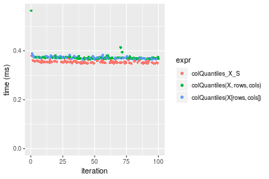
 Table: Benchmarking of colQuantiles_X_S() and rowQuantiles_X_S() on 1000x10 data (original and transposed). The top panel shows times in milliseconds and the bottom panel shows relative times.
| expr | min | lq | mean | median | uq | max | |
|---|---|---|---|---|---|---|---|
| 1 | colQuantiles_X_S | 347.737 | 350.8535 | 354.0595 | 352.988 | 356.3305 | 379.311 |
| 2 | rowQuantiles_X_S | 361.176 | 363.5325 | 368.9631 | 366.352 | 369.3885 | 529.790 |
| expr | min | lq | mean | median | uq | max | |
|---|---|---|---|---|---|---|---|
| 1 | colQuantiles_X_S | 1.000000 | 1.000000 | 1.000000 | 1.00000 | 1.000000 | 1.000000 |
| 2 | rowQuantiles_X_S | 1.038647 | 1.036138 | 1.042093 | 1.03786 | 1.036646 | 1.396717 |
Figure: Benchmarking of colQuantiles_X_S() and rowQuantiles_X_S() on 1000x10 data (original and transposed). Outliers are displayed as crosses. Times are in milliseconds.

> X <- data[["10x1000"]]
> rows <- sample.int(nrow(X), size = nrow(X) * 0.7)
> cols <- sample.int(ncol(X), size = ncol(X) * 0.7)
> X_S <- X[rows, cols]
> gc()
          used  (Mb) gc trigger  (Mb) max used  (Mb)
Ncells 3174781 169.6    5709258 305.0  5709258 305.0
Vcells 6072385  46.4   22343563 170.5 56666022 432.4
> probs <- seq(from = 0, to = 1, by = 0.25)
> colStats <- microbenchmark(colQuantiles_X_S = colQuantiles(X_S, probs = probs, na.rm = FALSE), `colQuantiles(X, rows, cols)` = colQuantiles(X,
+     rows = rows, cols = cols, probs = probs, na.rm = FALSE), `colQuantiles(X[rows, cols])` = colQuantiles(X[rows,
+     cols], probs = probs, na.rm = FALSE), unit = "ms")
> X <- t(X)
> X_S <- t(X_S)
> gc()
          used  (Mb) gc trigger  (Mb) max used  (Mb)
Ncells 3174772 169.6    5709258 305.0  5709258 305.0
Vcells 6082463  46.5   22343563 170.5 56666022 432.4
> rowStats <- microbenchmark(rowQuantiles_X_S = rowQuantiles(X_S, probs = probs, na.rm = FALSE), `rowQuantiles(X, cols, rows)` = rowQuantiles(X,
+     rows = cols, cols = rows, probs = probs, na.rm = FALSE), `rowQuantiles(X[cols, rows])` = rowQuantiles(X[cols,
+     rows], probs = probs, na.rm = FALSE), unit = "ms")
Table: Benchmarking of colQuantiles_X_S(), colQuantiles(X, rows, cols)() and colQuantiles(X[rows, cols])() on 10x1000 data. The top panel shows times in milliseconds and the bottom panel shows relative times.
| expr | min | lq | mean | median | uq | max | |
|---|---|---|---|---|---|---|---|
| 1 | colQuantiles_X_S | 8.012248 | 8.243809 | 9.089607 | 8.443760 | 9.317666 | 15.72662 |
| 2 | colQuantiles(X, rows, cols) | 7.978753 | 8.229190 | 11.738007 | 8.474258 | 9.434287 | 261.53323 |
| 3 | colQuantiles(X[rows, cols]) | 8.036511 | 8.270571 | 9.255518 | 8.487041 | 9.350547 | 16.61493 |
| expr | min | lq | mean | median | uq | max | |
|---|---|---|---|---|---|---|---|
| 1 | colQuantiles_X_S | 1.0000000 | 1.0000000 | 1.000000 | 1.000000 | 1.000000 | 1.000000 |
| 2 | colQuantiles(X, rows, cols) | 0.9958195 | 0.9982267 | 1.291366 | 1.003612 | 1.012516 | 16.629969 |
| 3 | colQuantiles(X[rows, cols]) | 1.0030282 | 1.0032464 | 1.018253 | 1.005126 | 1.003529 | 1.056485 |
Table: Benchmarking of rowQuantiles_X_S(), rowQuantiles(X, cols, rows)() and rowQuantiles(X[cols, rows])() on 10x1000 data (transposed). The top panel shows times in milliseconds and the bottom panel shows relative times.
| expr | min | lq | mean | median | uq | max | |
|---|---|---|---|---|---|---|---|
| 2 | rowQuantiles(X, cols, rows) | 8.068601 | 8.283373 | 8.699466 | 8.424089 | 8.919847 | 15.23229 |
| 1 | rowQuantiles_X_S | 8.072643 | 8.315941 | 9.143712 | 8.467600 | 9.180913 | 15.80287 |
| 3 | rowQuantiles(X[cols, rows]) | 8.126022 | 8.358648 | 9.244347 | 8.631372 | 9.439137 | 16.19782 |
| expr | min | lq | mean | median | uq | max | |
|---|---|---|---|---|---|---|---|
| 2 | rowQuantiles(X, cols, rows) | 1.000000 | 1.000000 | 1.000000 | 1.000000 | 1.000000 | 1.000000 |
| 1 | rowQuantiles_X_S | 1.000501 | 1.003932 | 1.051066 | 1.005165 | 1.029268 | 1.037459 |
| 3 | rowQuantiles(X[cols, rows]) | 1.007117 | 1.009087 | 1.062634 | 1.024606 | 1.058217 | 1.063387 |
Figure: Benchmarking of colQuantiles_X_S(), colQuantiles(X, rows, cols)() and colQuantiles(X[rows, cols])() on 10x1000 data as well as rowQuantiles_X_S(), rowQuantiles(X, cols, rows)() and rowQuantiles(X[cols, rows])() on the same data transposed. Outliers are displayed as crosses. Times are in milliseconds.

 Table: Benchmarking of colQuantiles_X_S() and rowQuantiles_X_S() on 10x1000 data (original and transposed). The top panel shows times in milliseconds and the bottom panel shows relative times.
| expr | min | lq | mean | median | uq | max | |
|---|---|---|---|---|---|---|---|
| 1 | colQuantiles_X_S | 8.012248 | 8.243809 | 9.089607 | 8.44376 | 9.317666 | 15.72662 |
| 2 | rowQuantiles_X_S | 8.072643 | 8.315941 | 9.143712 | 8.46760 | 9.180913 | 15.80287 |
| expr | min | lq | mean | median | uq | max | |
|---|---|---|---|---|---|---|---|
| 1 | colQuantiles_X_S | 1.000000 | 1.00000 | 1.000000 | 1.000000 | 1.0000000 | 1.000000 |
| 2 | rowQuantiles_X_S | 1.007538 | 1.00875 | 1.005952 | 1.002823 | 0.9853233 | 1.004849 |
Figure: Benchmarking of colQuantiles_X_S() and rowQuantiles_X_S() on 10x1000 data (original and transposed). Outliers are displayed as crosses. Times are in milliseconds.

> X <- data[["100x1000"]]
> rows <- sample.int(nrow(X), size = nrow(X) * 0.7)
> cols <- sample.int(ncol(X), size = ncol(X) * 0.7)
> X_S <- X[rows, cols]
> gc()
          used  (Mb) gc trigger  (Mb) max used  (Mb)
Ncells 3174977 169.6    5709258 305.0  5709258 305.0
Vcells 6117111  46.7   22343563 170.5 56666022 432.4
> probs <- seq(from = 0, to = 1, by = 0.25)
> colStats <- microbenchmark(colQuantiles_X_S = colQuantiles(X_S, probs = probs, na.rm = FALSE), `colQuantiles(X, rows, cols)` = colQuantiles(X,
+     rows = rows, cols = cols, probs = probs, na.rm = FALSE), `colQuantiles(X[rows, cols])` = colQuantiles(X[rows,
+     cols], probs = probs, na.rm = FALSE), unit = "ms")
> X <- t(X)
> X_S <- t(X_S)
> gc()
          used  (Mb) gc trigger  (Mb) max used  (Mb)
Ncells 3174971 169.6    5709258 305.0  5709258 305.0
Vcells 6217194  47.5   22343563 170.5 56666022 432.4
> rowStats <- microbenchmark(rowQuantiles_X_S = rowQuantiles(X_S, probs = probs, na.rm = FALSE), `rowQuantiles(X, cols, rows)` = rowQuantiles(X,
+     rows = cols, cols = rows, probs = probs, na.rm = FALSE), `rowQuantiles(X[cols, rows])` = rowQuantiles(X[cols,
+     rows], probs = probs, na.rm = FALSE), unit = "ms")
Table: Benchmarking of colQuantiles_X_S(), colQuantiles(X, rows, cols)() and colQuantiles(X[rows, cols])() on 100x1000 data. The top panel shows times in milliseconds and the bottom panel shows relative times.
| expr | min | lq | mean | median | uq | max | |
|---|---|---|---|---|---|---|---|
| 1 | colQuantiles_X_S | 10.18937 | 10.38272 | 11.47289 | 10.68613 | 11.26622 | 21.97929 |
| 2 | colQuantiles(X, rows, cols) | 10.40267 | 10.59949 | 11.56238 | 10.83319 | 11.45710 | 25.01436 |
| 3 | colQuantiles(X[rows, cols]) | 10.41228 | 10.58153 | 11.45298 | 10.83808 | 11.35463 | 22.18076 |
| expr | min | lq | mean | median | uq | max | |
|---|---|---|---|---|---|---|---|
| 1 | colQuantiles_X_S | 1.000000 | 1.000000 | 1.0000000 | 1.000000 | 1.000000 | 1.000000 |
| 2 | colQuantiles(X, rows, cols) | 1.020934 | 1.020878 | 1.0078004 | 1.013762 | 1.016942 | 1.138088 |
| 3 | colQuantiles(X[rows, cols]) | 1.021876 | 1.019149 | 0.9982649 | 1.014220 | 1.007847 | 1.009167 |
Table: Benchmarking of rowQuantiles_X_S(), rowQuantiles(X, cols, rows)() and rowQuantiles(X[cols, rows])() on 100x1000 data (transposed). The top panel shows times in milliseconds and the bottom panel shows relative times.
| expr | min | lq | mean | median | uq | max | |
|---|---|---|---|---|---|---|---|
| 1 | rowQuantiles_X_S | 10.50413 | 10.71388 | 11.97065 | 10.97342 | 11.71819 | 28.87060 |
| 2 | rowQuantiles(X, cols, rows) | 10.61135 | 10.82808 | 11.98220 | 11.14736 | 11.66477 | 24.07509 |
| 3 | rowQuantiles(X[cols, rows]) | 10.62854 | 10.85966 | 11.77734 | 11.14840 | 11.92261 | 22.28323 |
| expr | min | lq | mean | median | uq | max | |
|---|---|---|---|---|---|---|---|
| 1 | rowQuantiles_X_S | 1.000000 | 1.000000 | 1.0000000 | 1.000000 | 1.0000000 | 1.0000000 |
| 2 | rowQuantiles(X, cols, rows) | 1.010208 | 1.010659 | 1.0009654 | 1.015851 | 0.9954409 | 0.8338963 |
| 3 | rowQuantiles(X[cols, rows]) | 1.011844 | 1.013606 | 0.9838513 | 1.015945 | 1.0174450 | 0.7718312 |
Figure: Benchmarking of colQuantiles_X_S(), colQuantiles(X, rows, cols)() and colQuantiles(X[rows, cols])() on 100x1000 data as well as rowQuantiles_X_S(), rowQuantiles(X, cols, rows)() and rowQuantiles(X[cols, rows])() on the same data transposed. Outliers are displayed as crosses. Times are in milliseconds.

 Table: Benchmarking of colQuantiles_X_S() and rowQuantiles_X_S() on 100x1000 data (original and transposed). The top panel shows times in milliseconds and the bottom panel shows relative times.
| expr | min | lq | mean | median | uq | max | |
|---|---|---|---|---|---|---|---|
| 1 | colQuantiles_X_S | 10.18937 | 10.38272 | 11.47289 | 10.68613 | 11.26622 | 21.97929 |
| 2 | rowQuantiles_X_S | 10.50413 | 10.71388 | 11.97065 | 10.97342 | 11.71819 | 28.87060 |
| expr | min | lq | mean | median | uq | max | |
|---|---|---|---|---|---|---|---|
| 1 | colQuantiles_X_S | 1.00000 | 1.000000 | 1.000000 | 1.000000 | 1.000000 | 1.000000 |
| 2 | rowQuantiles_X_S | 1.03089 | 1.031896 | 1.043386 | 1.026885 | 1.040117 | 1.313537 |
Figure: Benchmarking of colQuantiles_X_S() and rowQuantiles_X_S() on 100x1000 data (original and transposed). Outliers are displayed as crosses. Times are in milliseconds.

> X <- data[["1000x100"]]
> rows <- sample.int(nrow(X), size = nrow(X) * 0.7)
> cols <- sample.int(ncol(X), size = ncol(X) * 0.7)
> X_S <- X[rows, cols]
> gc()
          used  (Mb) gc trigger  (Mb) max used  (Mb)
Ncells 3175193 169.6    5709258 305.0  5709258 305.0
Vcells 6117939  46.7   22343563 170.5 56666022 432.4
> probs <- seq(from = 0, to = 1, by = 0.25)
> colStats <- microbenchmark(colQuantiles_X_S = colQuantiles(X_S, probs = probs, na.rm = FALSE), `colQuantiles(X, rows, cols)` = colQuantiles(X,
+     rows = rows, cols = cols, probs = probs, na.rm = FALSE), `colQuantiles(X[rows, cols])` = colQuantiles(X[rows,
+     cols], probs = probs, na.rm = FALSE), unit = "ms")
> X <- t(X)
> X_S <- t(X_S)
> gc()
          used  (Mb) gc trigger  (Mb) max used  (Mb)
Ncells 3175187 169.6    5709258 305.0  5709258 305.0
Vcells 6218022  47.5   22343563 170.5 56666022 432.4
> rowStats <- microbenchmark(rowQuantiles_X_S = rowQuantiles(X_S, probs = probs, na.rm = FALSE), `rowQuantiles(X, cols, rows)` = rowQuantiles(X,
+     rows = cols, cols = rows, probs = probs, na.rm = FALSE), `rowQuantiles(X[cols, rows])` = rowQuantiles(X[cols,
+     rows], probs = probs, na.rm = FALSE), unit = "ms")
Table: Benchmarking of colQuantiles_X_S(), colQuantiles(X, rows, cols)() and colQuantiles(X[rows, cols])() on 1000x100 data. The top panel shows times in milliseconds and the bottom panel shows relative times.
| expr | min | lq | mean | median | uq | max | |
|---|---|---|---|---|---|---|---|
| 1 | colQuantiles_X_S | 2.663449 | 2.692945 | 2.754061 | 2.705303 | 2.726732 | 3.421134 |
| 3 | colQuantiles(X[rows, cols]) | 2.756835 | 2.780410 | 3.021965 | 2.794395 | 2.823256 | 11.221324 |
| 2 | colQuantiles(X, rows, cols) | 2.755981 | 2.778030 | 2.956400 | 2.798392 | 2.831595 | 11.446626 |
| expr | min | lq | mean | median | uq | max | |
|---|---|---|---|---|---|---|---|
| 1 | colQuantiles_X_S | 1.000000 | 1.000000 | 1.000000 | 1.000000 | 1.000000 | 1.000000 |
| 3 | colQuantiles(X[rows, cols]) | 1.035062 | 1.032479 | 1.097276 | 1.032932 | 1.035399 | 3.280001 |
| 2 | colQuantiles(X, rows, cols) | 1.034741 | 1.031595 | 1.073469 | 1.034410 | 1.038457 | 3.345857 |
Table: Benchmarking of rowQuantiles_X_S(), rowQuantiles(X, cols, rows)() and rowQuantiles(X[cols, rows])() on 1000x100 data (transposed). The top panel shows times in milliseconds and the bottom panel shows relative times.
| expr | min | lq | mean | median | uq | max | |
|---|---|---|---|---|---|---|---|
| 1 | rowQuantiles_X_S | 2.844951 | 2.861944 | 2.993162 | 2.877883 | 2.907040 | 4.646321 |
| 2 | rowQuantiles(X, cols, rows) | 2.937658 | 2.963849 | 3.198382 | 2.983258 | 3.034340 | 11.780869 |
| 3 | rowQuantiles(X[cols, rows]) | 2.936644 | 2.968400 | 3.265414 | 2.990714 | 3.056268 | 13.859673 |
| expr | min | lq | mean | median | uq | max | |
|---|---|---|---|---|---|---|---|
| 1 | rowQuantiles_X_S | 1.000000 | 1.000000 | 1.000000 | 1.000000 | 1.000000 | 1.000000 |
| 2 | rowQuantiles(X, cols, rows) | 1.032587 | 1.035607 | 1.068563 | 1.036615 | 1.043790 | 2.535526 |
| 3 | rowQuantiles(X[cols, rows]) | 1.032230 | 1.037197 | 1.090958 | 1.039206 | 1.051333 | 2.982935 |
Figure: Benchmarking of colQuantiles_X_S(), colQuantiles(X, rows, cols)() and colQuantiles(X[rows, cols])() on 1000x100 data as well as rowQuantiles_X_S(), rowQuantiles(X, cols, rows)() and rowQuantiles(X[cols, rows])() on the same data transposed. Outliers are displayed as crosses. Times are in milliseconds.

 Table: Benchmarking of colQuantiles_X_S() and rowQuantiles_X_S() on 1000x100 data (original and transposed). The top panel shows times in milliseconds and the bottom panel shows relative times.
| expr | min | lq | mean | median | uq | max | |
|---|---|---|---|---|---|---|---|
| 1 | colQuantiles_X_S | 2.663449 | 2.692945 | 2.754061 | 2.705303 | 2.726732 | 3.421134 |
| 2 | rowQuantiles_X_S | 2.844951 | 2.861944 | 2.993162 | 2.877883 | 2.907040 | 4.646321 |
| expr | min | lq | mean | median | uq | max | |
|---|---|---|---|---|---|---|---|
| 1 | colQuantiles_X_S | 1.000000 | 1.000000 | 1.000000 | 1.000000 | 1.000000 | 1.000000 |
| 2 | rowQuantiles_X_S | 1.068145 | 1.062756 | 1.086818 | 1.063793 | 1.066126 | 1.358123 |
Figure: Benchmarking of colQuantiles_X_S() and rowQuantiles_X_S() on 1000x100 data (original and transposed). Outliers are displayed as crosses. Times are in milliseconds.

R version 3.6.1 Patched (2019-08-27 r77078)
Platform: x86_64-pc-linux-gnu (64-bit)
Running under: Ubuntu 18.04.3 LTS

Matrix products: default
BLAS:   /home/hb/software/R-devel/R-3-6-branch/lib/R/lib/libRblas.so
LAPACK: /home/hb/software/R-devel/R-3-6-branch/lib/R/lib/libRlapack.so

locale:
 [1] LC_CTYPE=en_US.UTF-8       LC_NUMERIC=C
 [3] LC_TIME=en_US.UTF-8        LC_COLLATE=en_US.UTF-8
 [5] LC_MONETARY=en_US.UTF-8    LC_MESSAGES=en_US.UTF-8
 [7] LC_PAPER=en_US.UTF-8       LC_NAME=C
 [9] LC_ADDRESS=C               LC_TELEPHONE=C
[11] LC_MEASUREMENT=en_US.UTF-8 LC_IDENTIFICATION=C

attached base packages:
[1] stats     graphics  grDevices utils     datasets  methods   base

other attached packages:
[1] microbenchmark_1.4-6    matrixStats_0.55.0-9000 ggplot2_3.2.1
[4] knitr_1.24              R.devices_2.16.0        R.utils_2.9.0
[7] R.oo_1.22.0             R.methodsS3_1.7.1       history_0.0.0-9002

loaded via a namespace (and not attached):
 [1] Biobase_2.45.0       bit64_0.9-7          splines_3.6.1
 [4] network_1.15         assertthat_0.2.1     highr_0.8
 [7] stats4_3.6.1         blob_1.2.0           robustbase_0.93-5
[10] pillar_1.4.2         RSQLite_2.1.2        backports_1.1.4
[13] lattice_0.20-38      glue_1.3.1           digest_0.6.20
[16] colorspace_1.4-1     sandwich_2.5-1       Matrix_1.2-17
[19] XML_3.98-1.20        lpSolve_5.6.13.3     pkgconfig_2.0.2
[22] genefilter_1.66.0    purrr_0.3.2          ergm_3.10.4
[25] xtable_1.8-4         mvtnorm_1.0-11       scales_1.0.0
[28] tibble_2.1.3         annotate_1.62.0      IRanges_2.18.2
[31] TH.data_1.0-10       withr_2.1.2          BiocGenerics_0.30.0
[34] lazyeval_0.2.2       mime_0.7             survival_2.44-1.1
[37] magrittr_1.5         crayon_1.3.4         statnet.common_4.3.0
[40] memoise_1.1.0        laeken_0.5.0         R.cache_0.13.0
[43] MASS_7.3-51.4        R.rsp_0.43.1         tools_3.6.1
[46] multcomp_1.4-10      S4Vectors_0.22.1     trust_0.1-7
[49] munsell_0.5.0        AnnotationDbi_1.46.1 compiler_3.6.1
[52] rlang_0.4.0          grid_3.6.1           RCurl_1.95-4.12
[55] cwhmisc_6.6          rappdirs_0.3.1       labeling_0.3
[58] bitops_1.0-6         base64enc_0.1-3      boot_1.3-23
[61] gtable_0.3.0         codetools_0.2-16     DBI_1.0.0
[64] markdown_1.1         R6_2.4.0             zoo_1.8-6
[67] dplyr_0.8.3          bit_1.1-14           zeallot_0.1.0
[70] parallel_3.6.1       Rcpp_1.0.2           vctrs_0.2.0
[73] DEoptimR_1.0-8       tidyselect_0.2.5     xfun_0.9
[76] coda_0.19-3
Total processing time was 26.99 secs.
To reproduce this report, do:
html <- matrixStats:::benchmark('colRowQuantiles_subset')Copyright Dongcan Jiang. Last updated on 2019-09-10 20:49:41 (-0700 UTC). Powered by RSP.
<script> var link = document.createElement('link'); link.rel = 'icon'; link.href = "data:image/png;base64,iVBORw0KGgoAAAANSUhEUgAAACAAAAAgCAMAAABEpIrGAAAA21BMVEUAAAAAAP8AAP8AAP8AAP8AAP8AAP8AAP8AAP8AAP8AAP8AAP8AAP8AAP8AAP8AAP8AAP8AAP8AAP8AAP8AAP8AAP8AAP8AAP8AAP8AAP8AAP8AAP8AAP8AAP8AAP8AAP8AAP8AAP8AAP8AAP8AAP8AAP8AAP8AAP8AAP8AAP8BAf4CAv0DA/wdHeIeHuEfH+AgIN8hId4lJdomJtknJ9g+PsE/P8BAQL9yco10dIt1dYp3d4h4eIeVlWqWlmmXl2iYmGeZmWabm2Tn5xjo6Bfp6Rb39wj4+Af//wA2M9hbAAAASXRSTlMAAQIJCgsMJSYnKD4/QGRlZmhpamtsbautrrCxuru8y8zN5ebn6Pn6+///////////////////////////////////////////LsUNcQAAAS9JREFUOI29k21XgkAQhVcFytdSMqMETU26UVqGmpaiFbL//xc1cAhhwVNf6n5i5z67M2dmYOyfJZUqlVLhkKucG7cgmUZTybDz6g0iDeq51PUr37Ds2cy2/C9NeES5puDjxuUk1xnToZsg8pfA3avHQ3lLIi7iWRrkv/OYtkScxBIMgDee0ALoyxHQBJ68JLCjOtQIMIANF7QG9G9fNnHvisCHBVMKgSJgiz7nE+AoBKrAPA3MgepvgR9TSCasrCKH0eB1wBGBFdCO+nAGjMVGPcQb5bd6mQRegN6+1axOs9nGfYcCtfi4NQosdtH7dB+txFIpXQqN1p9B/asRHToyS0jRgpV7nk4nwcq1BJ+x3Gl/v7S9Wmpp/aGquum7w3ZDyrADFYrl8vHBH+ev9AUASW1dmU4h4wAAAABJRU5ErkJggg==" document.getElementsByTagName('head')[0].appendChild(link); </script>