-
Notifications
You must be signed in to change notification settings - Fork 11
Introduction
PyIBIS-AMI is a Python project containing Python packages, intended for use in developing/testing IBIS Algorithmic Modeling Interface (AMI) models. Currently, there is just one package included in the PyIBIS-AMI project, named pyibisami. The pyibisami package has been designed for the following 3 modes of operation:
Interactive use, from the PyLab command prompt.
To this end, classes have been created for the AMI model structure itself, as well as its initialization data, in order to encapsulate and store the data necessary for working with these models and obviate the need to continually retype redundant values at the PyLab command prompt. For instance, one can instantiate the AMIModelInitializer class, use it to initialize an instance of the AMIModel class, and then modify individual attributes, incrementally, re-initializing the model each time, in order to probe a new model's response to various initialization settings, without having to retype every piece of initialization data at every call of initialize.
So, for instance, a typical session at the PyLab command prompt might resemble this:
In [1]: import pyibisami.amimodel as ami
In [3]: theModel = ami.AMIModel('dll.so')
In [4]: initData = ami.AMIModelInitializer({'root_name' : 'myDLL', 'Mode' : 1})
In [5]: theModel.initialize(initData)
In [6]: h1 = theModel.initOut
In [8]: T = theModel.sample_interval
In [9]: t = [i * T for i in range(len(h1))]
In [12]: plot(t, h1)
Out[12]: [<matplotlib.lines.Line2D object at 0xb8218ac>]
In [13]: title('Model Impulse Response')
Out[13]: <matplotlib.text.Text object at 0xba8a2ec>
In [19]: xlabel('Time (s)')
Out[19]: <matplotlib.text.Text object at 0xbb2ba6c>
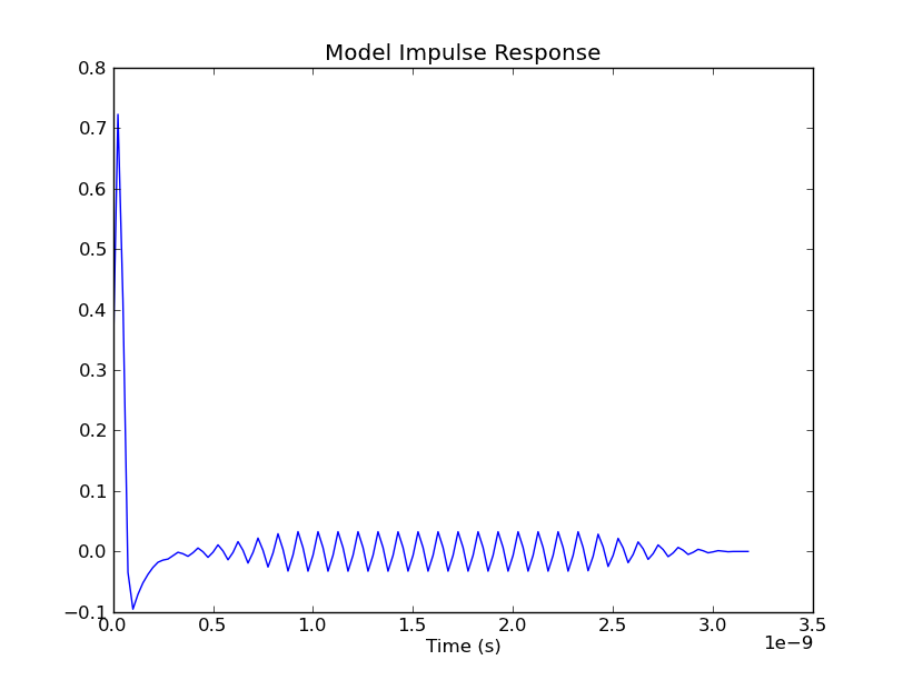
And the resultant plot might look something like this:

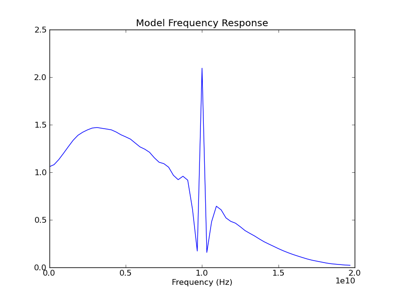
We weren't expecting that ringing in the impulse response. So, we take the Fast Fourier Transform (FFT) of it, in order to look at its spectral content:
In [20]: H1 = fft.fft(h1)
In [32]: cla()
In [33]: f = [i * (1/theModel.sample_interval) / len(t) for i in range(len(t) / 2)]
In [40]: plot(f, abs(H1[:len(H1)/2]))
Out[40]: [<matplotlib.lines.Line2D object at 0xb4bf0cc>]
In [41]: title('Model Frequency Response')
Out[41]: <matplotlib.text.Text object at 0xaf0448c>
In [42]: xlabel('Frequency (Hz)')
Out[42]: <matplotlib.text.Text object at 0xb4bd3ac>

That spike, at 10 GHz, is completely unexpected. The first thought that occurs to us is, "does it have something to do with the bit rate?" So, we quickly investigate this:
In [43]: theModel.bit_time
Out[43]: 1e-10
Aha! We were running at 10 Gbps. So, the spike could be related to our bit rate. In order to be sure, we change the bit rate and watch what happens to the spectrum:
In [44]: initData.bit_time = 2e-10
In [45]: theModel.initialize(initData)
In [46]: h2 = theModel.initOut
In [51]: H2 = fft.fft(h2)
In [52]: cla()
In [53]: plot(f, abs(H2[:len(H2)/2]))
Out[53]: [<matplotlib.lines.Line2D object at 0xaf040ac>]
In [54]: title('Model Frequency Response')
Out[54]: <matplotlib.text.Text object at 0xb31ec8c>
In [55]: xlabel('Frequency (Hz)')
Out[55]: <matplotlib.text.Text object at 0xb4bd3ac>

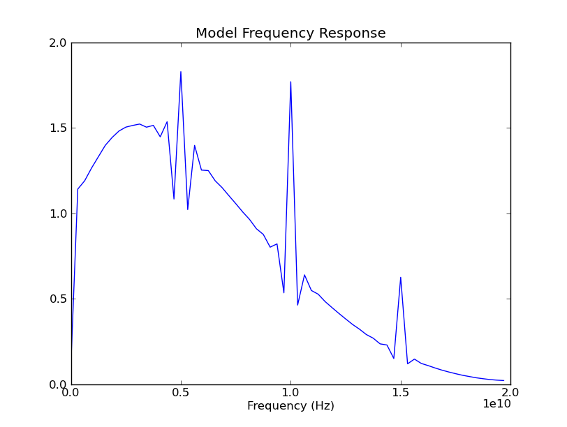
And our suspicions are confirmed, as the spectral spike has shifted to 5 GHz, following the change of bit rate to 5 Gbps. (The spikes at 10 and 15 GHz are, no doubt, the second and third harmonics of the 5 GHz fundamental. And the only reason we didn't see harmonics in the previous case is the second, at 20 GHz, was just off screen to the right.)
Indeed, myriad opportunities for further investigation exist, due to the fact that you are working from the PyLab command prompt and have all the power of Python and its various libraries (in particular, NumPy and SciPy) at your fingertips, while the model is executing and in scope.
The run_tests.py script has been provided, as part of the PyIBIS-AMI package, specifically to enable batch mode operation, as part of a larger, scripted/automated/unattended testing flow (i.e. - nightly regression testing). In order to support this mode of operation, run_tests.py has been designed to read the required testing actions from a separate file, written using a simple test specification grammar. (In fact, run_tests.py will run any number of test files against a particular model, and allow any number of parameter sweeps per test.) This grammar uses the EmPy Python templating language and produces XML as its final output. The resultant XML is made more user friendly, via association with the test_results.xsl XSLT style sheet, included in this package. If you'd like to view example run_tests.py output, point your browser to the test_results.xml file in the pyibisami installation directory, typically, located in the site-packages subdirectory of your personal Python installation, and findable, in any case, via the package __path__ attribute. So, for instance, from a PyLab prompt on my own Linux machine:
In [1]: import pyibisami
In [2]: pyibisami.__path__
Out[2]: '/home/dbanas/.local/lib/python2.7/site-packages/PyIBIS_AMI-0.4-py2.7.egg/pyibisami'
Note) For some reason, trying to view local XML/XSLT doesn't work on Chrome, although it works with every other browser I've tried.
Refer to the example tests/*.em and test_runs/*.run files, provided in the pyibisami installation directory, for examples of how to write test and parameter sweep files, respectively. And refer to the Test Specification Grammar page of this WiKi, for more details.
For quick help on the run_tests.py script:
$ ./run_tests.py -h
Usage: run_tests.py [options] [test1 [test2 ...]]

     Run a series of tests on a AMI model DLL file. If no tests are
specified on the command line, run all tests found in `test_dir'.     (See
`-t' option.)

Options:
  -h, --help            show this help message and exit
  -v, --version         Show program version info and exit.
{snip}
Note) The remaining operational mode described, below, does not yet function correctly. (Consider it the current "ToDo" list.)
This mode of operation requires that the Enthought Python Distribution (EPD) be installed and provides visual interactive model testing ability.