Matrix functions
These functions return and operate on native MATLAB matrices. They are the earliest part of the Toolbox (circa 1993) and their functionality has been superseded by a set of classes which also provide increased code readability and type safety.
You should use these matrix functions if:
- you want to strip away the complexity of classes, methods and overloaded operators to expose the underlying concepts, eg. for teaching.
- efficiency is a concern, the classes have some additional computational overhead
- you want to generate code using MATLAB codegen tools
- you want to use Simulink, the signals can be scalars or matrices, but not (yet) objects
- you want to use Octave (Octave 5 supports classes but the supported syntax is not entirely the same as MATLAB)
We use orthogonal rotation matrices – belonging to the groups SO(2) or SO(3)– or homogeneous transformation matrices –belonging to the groups SE(2) or SE(3). These are matrices with particular structure and properties – a subset of all possible real matrices.
A sequence of matrices, perhaps representing some rotating or translating body, is represented by a stack of matrices, a 3-dimensional matrix, and we use the third index to denote the position in the sequence.
Jump to description of functions for operations in 2D or 3D.
Many problems in robotics, particularly in mobile robotics, can be considered in terms of position and orientation in the plane. In 2D:
- position is defined by two quantities, typically denoted x and y.
- orientation is defined by one angle, typically denoted θ.
Orientation in 2D can be represented by a subset of 2×2 matrices that belong to the special orthogonal group of order 2 which in mathematical shorthand is written as SO(2). These matrices have special properties:
- determinant equals +1
- inverse is given by the transpose
To create such a matrix representing a rotation of 45 degrees is
>> R = rot2(45, 'deg')
R =
    0.7071   -0.7071
    0.7071    0.7071

>> whos R
  Name      Size            Bytes  Class     Attributes
  R         2x2                32  double
which is a native MATLAB real matrix.
We can think of this matrix as defining a new coordinate frame, rotated counter-clockwise, with respect to the world coordinate frame. To draw that frame is simply
>> trplot2(R)or animate the motion from the world frame to the rotated frame with
>> tranimate2(R)
We can interpolate between two orientations
    R1 = rot2(20, 'deg')
    R2 = rot2(90, 'deg')
    R = trinterp(R1, R2, 0.5)
where the 0.5 indicates a rotation half way between the initial and final rotations. This parameter can vary between 0, which would return R1 and 1 which would return R2.
We can return a sequence of rotation matrices
>> R = trinterp(R1, R2, 0:0.05:1);
>> whos R
  Name      Size              Bytes  Class     Attributes
  R         2x2x21              672  double
which is a sequence of twenty one 2×2 rotation matrices smoothly changing from R1 to R2.
Consider a coordinate frame {A}
>> A = rot2(45, 'deg')
A =
    0.7071   -0.7071
    0.7071    0.7071
>> trplot2(A, 'frame', 'A')
and a point defined with respect to the world
>> P = [0 1]'
P =
     0
     1
>> plot_point(P, 'label', 'P')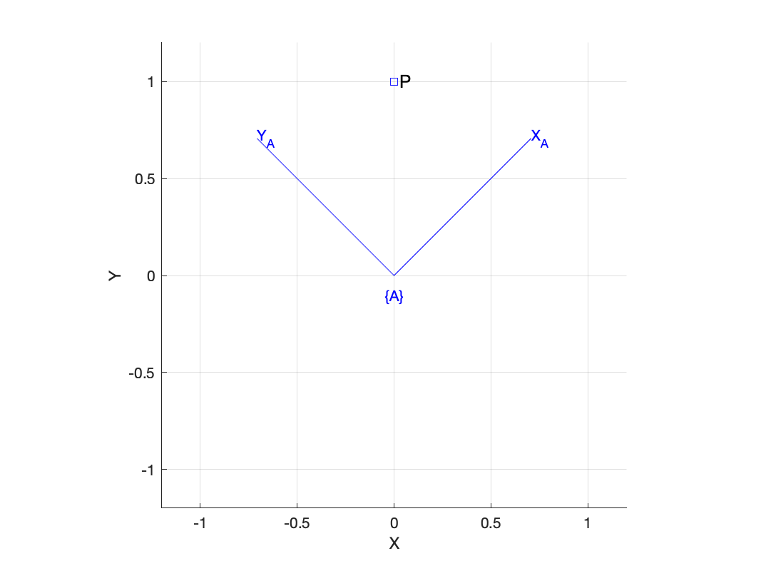
Now the position of the point with respect to frame {A} is
>> A'*P
ans =
    0.7071
    0.7071
which can be verified by inspection.
If we take the matrix logarithm of a rotation matrix we find
>> logm(A)
ans =
         0   -0.7854
    0.7854         0
we obtain a skew-symmetric matrix with a single unique element
>> vex(ans)
ans =
    0.7854
which is π/4 the rotation angle. In fact we can create a rotation matrix by exponentiating a skew-symmetric matrix
>> trexp2( skew(pi/4) )
ans =
    0.7071   -0.7071
    0.7071    0.7071
where trexp2 is an efficient version of matrix exponentiation for skew-symmetric matrices. The skew-symmetric matrix is referred to as the Lie algebra, mathematical group so(2), of the Lie group SO(2).
To represent position (as well as rotation) we need to use a slightly bigger matrix: a 3×3 homogeneous transformation matrix. To represent a displacement of 2 in the x-direction and 3 in the y-direction is simply
>> T = transl2([2, 3])
T =
     1     0     2
     0     1     3
     0     0     1
which represents the pose of a coordinate frame which we can show graphically
We can extract the translational component by
>> transl2(T)
ans =
     2
     3
Now in the general case, the coordinate frame attached to our object of interest will have an arbitrary translation and rotation which can be obtained by multiplying together the relevant homogeneous transformation matrices
>> A = transl2([2 3]) * trot2(30, 'deg')
A =
    0.8660   -0.5000    2.0000
    0.5000    0.8660    3.0000
         0         0    1.0000
which, reading left to right, is a translation by 2 in the x-direction and 3 in the y-direction then a rotation by 30 degrees (the function trot2 is like rot2 but it returns a 3×3 homogeneous transformation matrix rather than a 2×2 rotation matrix, with the translational part set to zero).
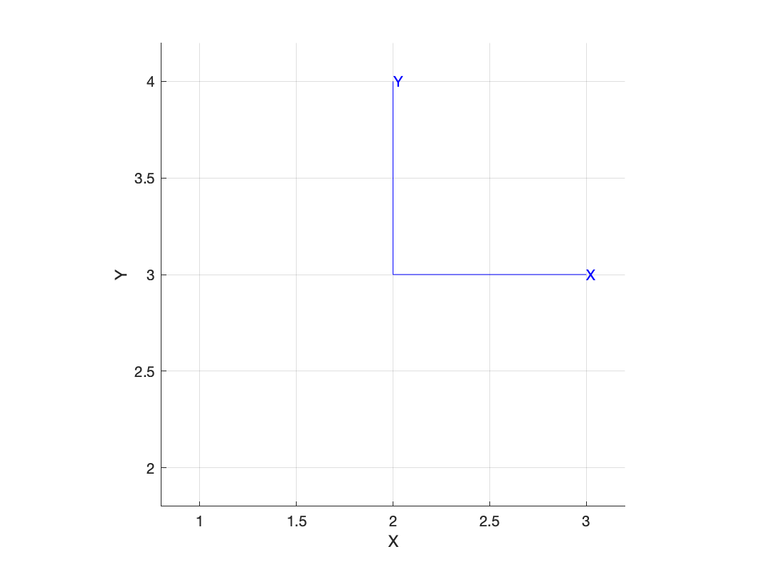
We can plot this frame
>> trplot2(A, 'frame', 'A')Consider a point defined with respect to the world frame
>> P = [2 4]'
P =
     2
     4
>> plot_point(P, 'label', 'P')
Now the position of the point with respect to the frame {A} is
>> inv(A)*[P; 1]   % convert P to homogeneous form
ans =
    0.5000
    0.8660
    1.0000
which is a homogeneous vector -- the equivalent Euclidean vector is simply the first two elements, and this result can be easily verified from the figure above. Note that the inverse of an SE(2) matrix is the regular matrix inverse, not the transpose (that trick only applies to orthogonal matrices).
To handle the conversion to and from homogeneous vector format we can use some Toolbox helper functions
>> h2e(inv(A)*e2h(P)
ans =
    0.5000
    0.8660
where h2e and e2h convert between Euclidean and homogeneous coordinates. Even simpler is
>> homtrans(inv(A), P)
ans =
    0.5000
    0.8660
which applies the first argument, an SE(2) transformation, to the point P. Note that in all these examples if P was a set of points (one point per column) then the result will be a set of transformed points, one per column.
If we take the matrix logarithm of a rotation matrix we find
>> logm(A)
ans =
         0   -0.7854
    0.7854         0
we obtain a skew-symmetric matrix with a single unique element
>> vex(ans)
ans =
    0.7854
which is π/4 the rotation angle. In fact we can create a rotation matrix by exponentiating a skew-symmetric matrix
>> trexp2( skew(pi/4) )
ans =
    0.7071   -0.7071
    0.7071    0.7071
where trexp2 is an efficient version of matrix exponentiation for skew-symmetric matrices. The skew-symmetric matrix is referred to as the Lie algebra, mathematical group so(2), of the Lie group SO(2).
Many problems in physics and robotics involve objects in everyday 3D space. For this we need to consider the more complicated case of orientation in 3D
- position is defined by three quantities, typically denoted x, y and z.
- orientation is defined by three angles, and there many options for denoting these.
Orientation in 3D can be represented by a subset of 3x3 matrices that belong to the special orthogonal group of order 3 which in mathematical shorthand is written as SO(3). These matrices have special properties:
- determinant equals +1
- inverse is given by the transpose
>> R = rotx(45, 'deg')
R =
    1.0000         0         0
         0    0.7071   -0.7071
         0    0.7071    0.7071

>> whos R
  Name      Size            Bytes  Class     Attributes
  R         3x3                72  double
which is a native MATLAB real matrix.
We can think of this matrix as defining a new coordinate frame, rotated about the world coordinate frame's x-axis. To draw that frame is simply
>> trplot(R)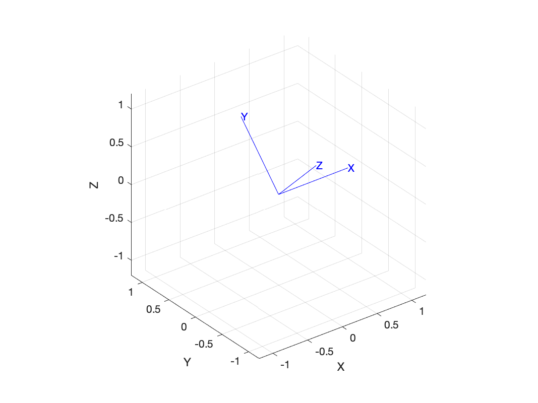
or animate the motion from the world frame to the rotated frame with
>>> tranimate(R) and since we are rotating about the x-axis it doesn't move.
Just as for the 2D-case we can interpolate between two orientations
>> R1 = rotx(20, 'deg')
>> R2 = roty(90, 'deg')
>> R = trinterp(R1, R2, 0.5)
where the 0.5 indicates a rotation half way between the initial and final rotations. This parameter can vary between 0, which would return R1 and 1 which would return R2.
We can return a sequence of rotation matrices
>> R = trinterp(R1, R2, 0:0.05:1);
>> whos R
  Name      Size              Bytes  Class     Attributes
  R         3x3x21              672  double
which is a sequence of twenty one 3×3 rotation matrices smoothly changing from R1 to R2.
If we take the matrix logarithm of a rotation matrix we find
>> trlog(R1)
ans =
         0         0         0
         0         0   -0.3491
         0    0.3491         0
we obtain a skew-symmetric matrix with three unique elements
>> vex(ans)
ans =
    0.3491
         0
         0
>> ans*180/pi
ans =
   20.0000
         0
         0
which is the rotation about the x-, y- and z-axes respectively. In fact we could create a rotation matrix by exponentiating a skew-symmetric matrix
>> trexp( skew([0 pi/4 0]) )
ans =
    0.7071         0    0.7071
         0    1.0000         0
   -0.7071         0    0.7071

>> roty(pi/4)
ans =
    0.7071         0    0.7071
         0    1.0000         0
   -0.7071         0    0.707
in this case creating a rotation of π/4 about the y-axis (second element of the vector).
Note that trlog and trexp are efficient versions of matrix logarithm and exponentiation for matrices of this type. The skew-symmetric matrix is referred to as the Lie algebra, mathematical group so(3), of the Lie group SO(3).
Given a homogeneous transformation matrix
>> T = trotx(30, 'deg')
T =
    1.0000         0         0         0
         0    0.8660   -0.5000         0
         0    0.5000    0.8660         0
         0         0         0    1.0000
we can extract the 3×3 rotation matrix by
>> R = t2r(T)
R =
    1.0000         0         0
         0    0.8660   -0.5000
         0    0.5000    0.8660
and conversely we can convert a 3×3 rotation matrix to a 4×4 homogeneous transformation matrix with zero translation by
>> r2t(R)
ans =
    1.0000         0         0         0
         0    0.8660   -0.5000         0
         0    0.5000    0.8660         0
         0         0         0    1.0000
We can add a translation component expressed as a 3×1 vector
>> T = rt2tr(R, [1 2 3]')
T =
    1.0000         0         0    1.0000
         0    0.8660   -0.5000    2.0000
         0    0.5000    0.8660    3.0000
         0         0         0    1.0000
or decompose a 4×4 homogeneous transformation matrix to a 3×3 rotation matrix and a 3×1 translation vector
>> [R,t] = tr2rt(T)
R =
    1.0000         0         0
         0    0.8660   -0.5000
         0    0.5000    0.8660
t =
     1
     2
     3
These functions all operate on sequences expressed as 3-dimensional matrices.
Sometimes we need to test if a MATLAB variable is of a particular type and we can use
>> ishomog(T)
ans =
  logical
   1
>> isrot(T)
ans =
  logical
   0
>> isrot(R)
ans =
  logical
   1
>> isvec(t)
ans =
  logical
   1
Analagous functions with a 2 suffix can be used for the 2D case.
Euclidean translation is represented by a 3×1 vector
>> t = [1 2 3]'
t =
     1
     2
     3
and can be converted to a 4×1 homogeneous vector
>> e2h(t)
ans =
     1
     2
     3
     1
which allows it to be premultiplied by a 4×4 homogeneous transformation matrix. The result will be another 4×1 homogeneous vector which can be converted to Euclidean form by
>> h2e(ans)
ans =
     1
     2
3A common operation is to build Lie algebra generator matrices. For rotation these are 3×3 skew-symmetric matrices belonging to the group so(3)
>> S1 = skew([1 2 3])
S1 =
     0    -3     2
     3     0    -1
    -2     1     0
a mapping from R3 to R3×3.
An augmented skew-symmetric matrices belonging to the group se(3)
>> S2 = skewa([1 2 3 4 5 6])
S2 =
     0    -6     5     1
     6     0    -4     2
    -5     4     0     3
     0     0     0     0
a mapping from R6 to R4×4. These matrices, also known as Lie group generator matrices, have particular structure:
- a zero diagonal
- singular, ie. determinant is zero
The inverse operation is
>> vex(S1)
ans =
     1
     2
     3
>> vexa(S2)
ans =
     1
     2
     3
     4
     5
     6
which are mappings from R3×3 to R3, and from R4×4 to R6 respectively.
Most interestingly the exponential of these matrices are Lie group matrices representing pose, for example
>> trexp( skew([0.3 0 0]) )
ans =
    1.0000         0         0
         0    0.9553   -0.2955
         0    0.2955    0.9553
is a rotation about of 0.3 radians about the x-axis.
The inverse is also true
>> R = roty(0.7)
R =
    0.7648         0    0.6442
         0    1.0000         0
   -0.6442         0    0.7648
>> vex(trlog(R))
ans =
         0
    0.7000
         0
The functions skew, skewa, vex and vexa operated on matrices for the 2D and 3D case. For exponentiation and logarithm the 2D-dimensional equivalents are trlog2, trexp2.
trchain stuff