Classes

Classes

The Spatial Math Toolbox matrix functions, the oldest part of the Toolbox, use native MATLAB matrices to represent position, orientation and pose. However this has a number of limitations:

• there is no type safety, MATLAB allows us to add two SE(2) matrices but that is not a valid operation on the SE(2) group.
• type introspection, a 3×3 matrix could represent an SE(2) pose or an SO(3) rotation.
• function names vary depending on whether you are working in 2D or 3D.
• a sequence of poses is a matrix with 3 indices which is notationally clumsy, eg. T(:,:,i).
• for code debugging the type of the object is clearly displayed in the workspace window.

To address these issues the Toolbox introduces a family of classes to represent these important mathematical objects:

    RTBPose (abstract handle class)
       |
       +--SO2
       |   |
       |   +-- SE2
       |
       +--SO3
           |
           +--SE3
       
    UnitQuaternion
    Quaternion
    Twist

The classes, derived from RTBPose, are designed to be substantially backward compatible with the native matrix functions.

2D

Many problems in robotics, particularly in mobile robotics, can be considered in terms of position and orientation in the plane. In 2D:

• position is defined by two quantities, typically denoted x and y.
• orientation is defined by one angle, typically denoted θ.

Orientation SO(2)

Orientation in 2D can be represented by an instance object of the SO2 class which contains internally a 2×2 matrices that belong to the special orthogonal group of order 2 which in mathematical shorthand is written as SO(2). These matrices have special properties:

• determinant equals +1
• inverse is given by the transpose

To create such a matrix representing a rotation of 45 degrees is

>> R = SO2(45, 'deg')
R =
    0.7071   -0.7071
    0.7071    0.7071

>> whos R
  Name      Size            Bytes  Class    Attributes
  R         1x1                32  SO2 

which is a MATLAB object -- an instance of the SO2 class. The result appears identical to that obtained using the rot2 function.

It is important to remember that R is an object not a matrix. A regular MATLAB matrix can be obtained by

>> double(R)   % or R.R
ans =
    0.7071   -0.7071
    0.7071    0.7071
>> whos ans
  Name      Size            Bytes  Class     Attributes
  ans       2x2                32  double 

We can think of this object as defining a new coordinate frame, rotated counter-clockwise, with respect to the world coordinate frame. To draw that frame is simply

>> R.plot()

using C++/Java style dot notation or we can write it in more conventional MATLAB functional notation as

>> plot(R)

Note that, just as for a 2×2 matrix, we can also write

>> trplot2(R)

which has the same semantics as would be used with a native MATLAB matrix, but with the added advantage of type safety. In this case trplot2 is a method of the SO2 class.

We can animate the motion from the world frame to the rotated frame with

>>> R.animate()

We can interpolate between two orientations

    R1 = SO2(20, 'deg')
    R2 = SO2(90, 'deg')
    R = interp(R1, R2, 0.5)   % or R1.interp(R2, 0.5)

where the 0.5 indicates a rotation half way between the initial and final rotations. This parameter can vary between 0, which would return R1 and 1 which would return R2.

We can return a sequence of rotation matrices

>> R = interp(R1, R2, 0:0.05:1);
>> whos R
  Name      Size              Bytes  Class     Attributes
  R         1x21              672  SO2            

which is a sequence of twenty one SO2 objects smoothly changing from R1 to R2.

Consider an arbitrary rotation defining a frame {A} and point defined with respect to the world frame

>> A = SO2(45, 'deg')
A =
    0.7071   -0.7071
    0.7071    0.7071
>> A.plot('frame', 'A')
>> P = [0 1]'
P =
     0
     1
>> plot_point(P, 'label', 'P')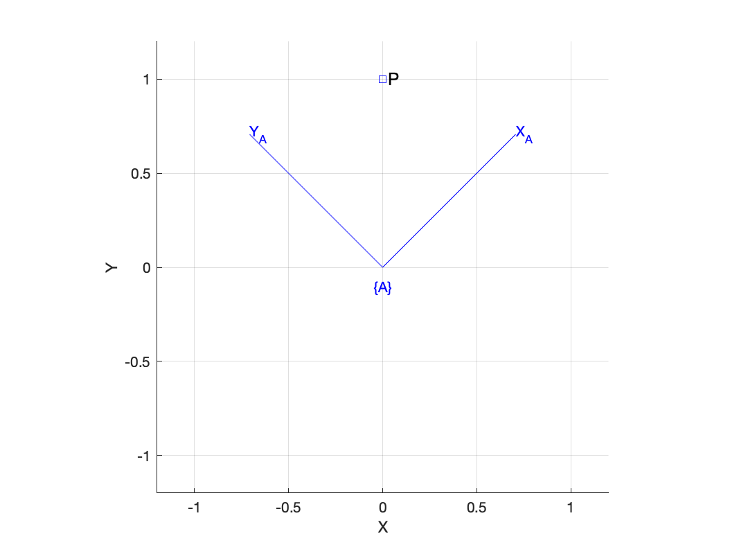

Now the position of the point with respect to the frame {A} is

>> A'*P
ans =
    0.7071
    0.7071

which can be easily verified. In this case the multiplication operator has been overloaded by the SO2 class.

Note that if we add two SO2 objects

>> A+A
ans =
    1.4142   -1.4142
    1.4142    1.4142

the result will not be an SO2 object because addition is not defined for the SO(2) group. The result will instead be a regular MATLAB matrix.

>> whos ans
  Name      Size            Bytes  Class     Attributes
  ans       2x2                32  double

Other arithmetic operators are supported, for example

>> A^2
ans = 
         0        -1
         1         0

is equivalent to A*A which represents a rotation of 45deg followed by a rotation of 45deg for a total rotation of 90deg.

>> inv(A)
ans = 
    0.7071    0.7071
   -0.7071    0.7071

is the inverse of A which for an SO(2) matrix is its transpose.

>> A/A
ans = 
         1         0
         0         1

is the same as A*inv(A) which is the identity matrix as expected.

Logical operators are also supported, eg.

>> A==A
ans =
  logical
   1

which tests for equality between all the matrix elements.

Finally, sometimes for the purposes of example it is nice to have a random rotation matrix

>> SO2.rand
ans = 
    0.6861   -0.7275
    0.7275    0.6861

Pose SE(2)

To represent position (as well as rotation) we use an instance object of the SE2 class which contains internally a 3&tmes;3 homogeneous transformation matrix. To represent a displacement of 2 in the x-direction and 3 in the y-direction is simply

>> T = SE2(2, 3)
T =
     1     0     2
     0     1     3
     0     0     1

which represents the pose of a coordinate frame which we can show graphically by

>> T.plot()   % or plot(T)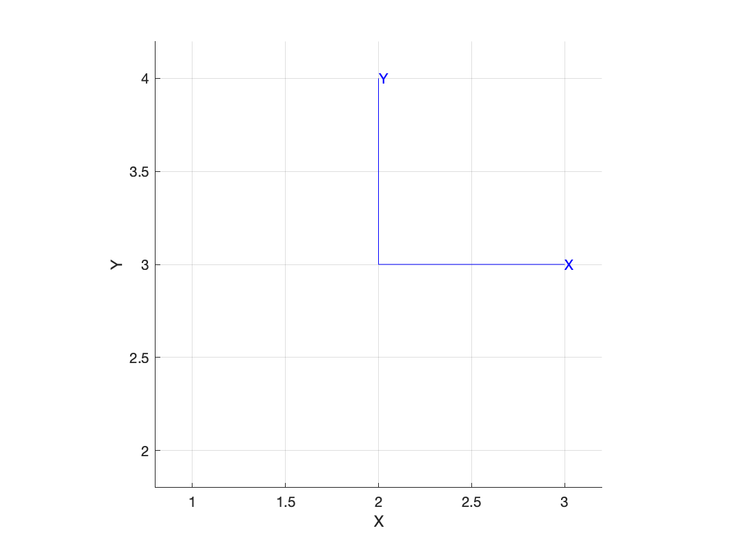

We can extract the translational component by

>> T.t
ans =
     2
     3

Note that for compatability purposes we could also use the transl2 method.

Now in the general case, the coordinate frame attached to our object of interest will have an arbitrary translation and rotation which can be specified in the constructor as

>> SE2(2, 3, 30, 'deg')    % or SE2( [2 3 30], 'deg')
ans = 
    0.8660   -0.5000         2
    0.5000    0.8660         3
         0         0         1

which is a translation by 2 in the x-direction and 3 in the y-direction then a rotation by 30 degrees.

Consider a point defined with respect to the frame {A}

>> A.plot('frame', 'A')
>> P = [2 4]'
P =
     2
     4
>> plot_point(P, 'label', 'P')

which is shown above

Now the position of the point with respect to the world frame is

>> inv(A)*P
ans =
    0.5000
    0.8660

which is a Euclidean vector. Note that the SE2 class has done all the work of is simply the first two elements, and this result can be easily verified from the figure above.

3D

Many problems in physics and robotics involve objects in everyday 3D space. For this we need to consider the more complicated case of orientation in 3D

• position is defined by 3 quantities, typically denoted x, y and z.
• orientation is defined by 3 angles, and there many options for denoting these.

Orientation SO(3)

Orientation in 3D can be represented by a subset of 3x3 matrices that belong to the special orthogonal group of order 3 which in mathematical shorthand is written as SO(3). These matrices have special properties:

• determinant equals +1
• inverse is given by the transpose

>> R = SO3.Rx(45, 'deg')
R =
    1.0000         0         0
         0    0.7071   -0.7071
         0    0.7071    0.7071

>> whos R
  Name      Size            Bytes  Class     Attributes
  R         1x1                72  SO3              

which is a MATLAB object -- an instance of the SO3 class. The result is appears identical to that obtained using the rotx function.

We can think of this object as defining a new coordinate frame, rotated about the world coordinate frame's x-axis. To draw that frame is simply

>> R.plot()    % or plot(R)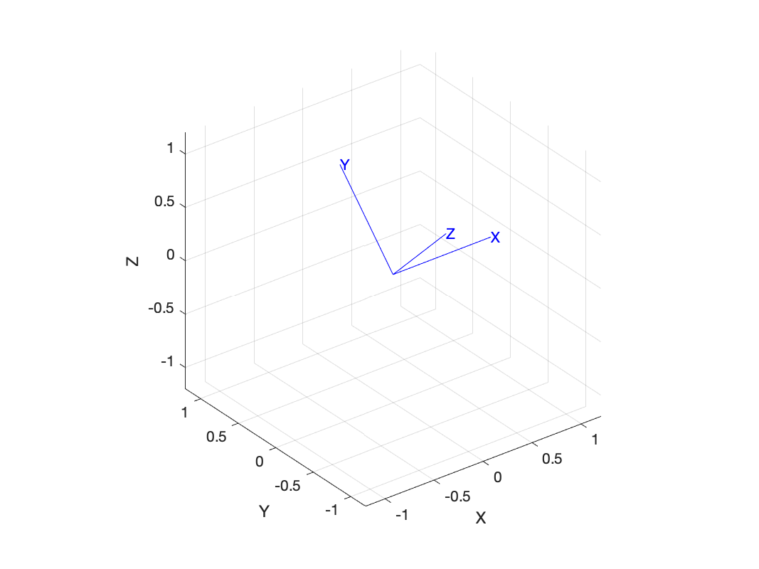

or animate the motion from the world frame to the rotated frame with

>> R.animate()    % or animate(R)

and since we are rotating about the x-axis it doesn't move.

Just as for the 2D-case we can interpolate between two orientations

>> R1 = SO3.Rx(20, 'deg')
>> R2 = SO3.Ry(90, 'deg')
>> R = interp(R1, R2, 0.5)    % or R1.interp(R2, 0.5)

where the 0.5 indicates a rotation half way between the initial and final rotations. This parameter can vary between 0, which would return R1 and 1 which would return R2.

We can return a sequence of rotation matrices

>> R = interp(R1, R2, 0:0.05:1);    % or R1.interp(R2, 0:0.05:1)
>> whos R
  Name      Size              Bytes  Class     Attributes

  R         1x21             1512  SO3  

which is a sequence of twenty one SO3 orientation objects smoothly changing from R1 to R2.

RPY angles Euler angles rotvec OA vectors

UnitQuaternion

Pose SE(3)