Python plotting

Python plotting with mjolnir.py

The mjolnir (THOR/mjolnir/) plotting scripts are written for Python 3 (compatibility with Python 2 still needs to be tested). Most dependencies are pretty standard for science: numpy, matplotlib, and scipy. Additionally, you'll need to install h5py:

$ pip3 install h5py

or

$ conda install h5py

h5py is simply a Python package that allows easy interaction with hdf5 files (THOR's standard output format).

mjolnir.py is set up as an executable for command line, but you'll need to add the path to your environment file. In bash, add the line

export PATH="$PATH:<path to thor>/mjolnir"

to your ~/.bashrc or ~/.bash_profile file, replacing <path to thor> with the actual path to the repository on your system. Probably not the smartest or most pythonic way of setting this up but one thing at a time please. Once that is done, the command to make a plot looks like

$ mjolnir <options> <type of plot>

For example,

$ mjolnir -i 0 -l 10 -f awesome_results -s coolest_planet Tver

where -i, -l, -f, and -s are options flags and Tver is a plot type. The available options flags are

 -i / --initial_file <N>       number of first output file to open
 -l / --last_file <N>          number of last output file to open
 -f / --file <string>          folder containing results
 -s / --simulation_ID <string> name of planet (used in naming of output files)
 -p / --pressure_lev <N>       pressure level to use in horizontal plots (mbar units)
 -pmin / --pressure_min <N>    pressure minimum for vertical plots (mbar units)
 -slay / --split_layer <N>     splits conservation data into "weather" and "deep" layers at this pressure (mbar units)

mjolnir averages the data over time for the entire range of files read in. So with -i 0 and -l 10, files 0-10 will all be read in, and the plotted quantities will be averaged over all 11 snapshots in time. If you want to plot one instant in time, just set -i and -l to the same value. The averaging process can get quite long because the data is interpolated in many ways before averaging. Be careful if you are passing mjolnir more than ~50 output files.

There are three basic types of plot mjolnir can make (plus a few other special ones): vertical, horizontal, and profile. Vertical plots are averaged zonally and temporally, resulting in contours on a latitude vs pressure grid. Horizontal plots are averaged only temporally, and plotted at a given pressure level on a latitude vs longitude grid. Profile plots show quantities along single columns or average columns, as a function of pressure.

The -p option is used only by the horizontal plot types and is simply the desired pressure level to be viewed. The -pmin option is used only by the vertical plot types and is just the lowest pressure level to be plotted. For vertical plots, mjolnir will plot a dashed line representing the maximum pressure at the top of the model--thus data plotted above this line requires some extrapolation and should be viewed skeptically.

Current vertical plot types are

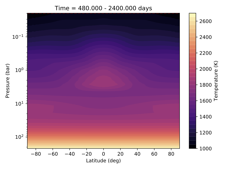
 Tver                           time- and zonally-averaged temperature
 uver                           time- and zonally-averaged zonal wind speed
 wver                           time- and zonally-averaged vertical wind speed
 PTver                          time- and zonally-averaged  potential temperature
 PVver                          time- and zonally-averaged  potential vorticity
 stream                         time- and zonally-averaged mass streaming function

An example of time- and zonally-averaged vertical plots are below. These show the temperature and zonal wind for the deep hot jupiter benchmark:

Current horizontal plot types are

 Tulev                          time-averaged temperature and horizontal wind along a pressure surface
 ulev                           time-averaged zonal and meridional winds along a pressure surface   
 PVlev                          time-averaged potential vorticity along a pressure surface
 RVlev                          time-averaged relative vorticity along a pressure surface
 tracer                         time-averaged molecular abundances along a pressure surface

Current profile plot types are

  TP                            temperature-pressure profiles drawn from all over the grid
  wprof                         vertical wind vs pressure averaged over 4 quadrants (useful for synchronous rotation)