Time Complexities

Introduction

Thinking of an efficient algorithm to solve a problem is one of the hardest tasks in competitive programming. Assessing your algorithm's efficiency is of upmost importance. This is where Time complexities are useful. They help us decide whether certain algorithms can solve the problem within the required time and space constraints. Time Complexity is one of the most important metrics of comparison for Algorithms.

For example consider two different sorting algorithms, bubble and quick sort. Bubble sort has a time complexity of O(N^2) whereas Quick Sort has a complexity of O(NlogN). Thus, we conclude that quick sort is more efficient than bubble sort. We will get into Big O notation later in this tutorial.

Observation

Let's look at an example code,

int func(int n)
{
    int sum=0;              //line 1
    for(int i=0;i<n;i++)    //line 2
        sum += i;           //line 3
    return sum;             //line 4
}

Let us now compute the number of times a statement is executed for each call of the function.

Line 1 and Line 4 are single statements and hence execute in one unit of time each.

Line 2 has a for loop which executes two statements, a check statement and an increment statement. The check statement runs exactly n+1 times (It stops once the condition is false). The increment statement runs for exactly n times. This line contributes 2n + 1 to the total runtime.

Line 3 has two operations, addition an assignment. Each of these operations takes 1 unit time each. Since the loop runs n times, this line contributes 2n to the total runtime.

So, the total runtime can be written as a function of the input size n. The function would be

We can see that the function is linear with respect to the input size n.

Asymptotic Notations

Let us dive into the different notations used for Algorithmic Complexities. There are three important notations we will look into.

Big Omega

Ω-notation provides an asymptotic lower bound. For a given function g(n), we denote Ω(g(n)) the set of functions

The graph shows that the function g ( n ) forms a lower bound for the function f ( n ). Consider,

Since,

The function g ( n ) can be said to be a lower bound of f ( n ). We can then say that,

In summary Ω(N) means it takes at least N steps.

Big Theta

Θ-notation provides an asymptotic tight bound. For a given function g(n), we denote Θ(g(n)) the set of functions

The graph shows that the function g ( n ) forms both the upper and lower bound for the function f ( n ) with the right constants c1 and c2. Consider,

The function g ( n ) can be called an asymptotic tight bound of f ( n ). We can then say that,

Big O

Ο-notation provides an asymptotic upper bound. For a given function g(n), we denote Ο(g(n)) the set of functions

In summary Ο(N) means it takes at most N steps. In general we use the Big O notation for analyzing algorithms because it gives us an upper bound, and we are mostly concerned with the worst case scenarios.

Let's look an example code. Consider that this code contains three different blocks which run sequentially , one after the other.

block 1 // runs in linear time
block 2 // runs in quadratic time
block 3 // runs in constant time

Now to calculate the overall time complexity of the above block of code, we can write the time function as the sum of runtimes of the individual blocks of code. That function would look like,

This can be expanded as,

Since the Big O complexity gives us an upper bound, we can reduce that to,

This equation ultimately boils down to

Common Complexities

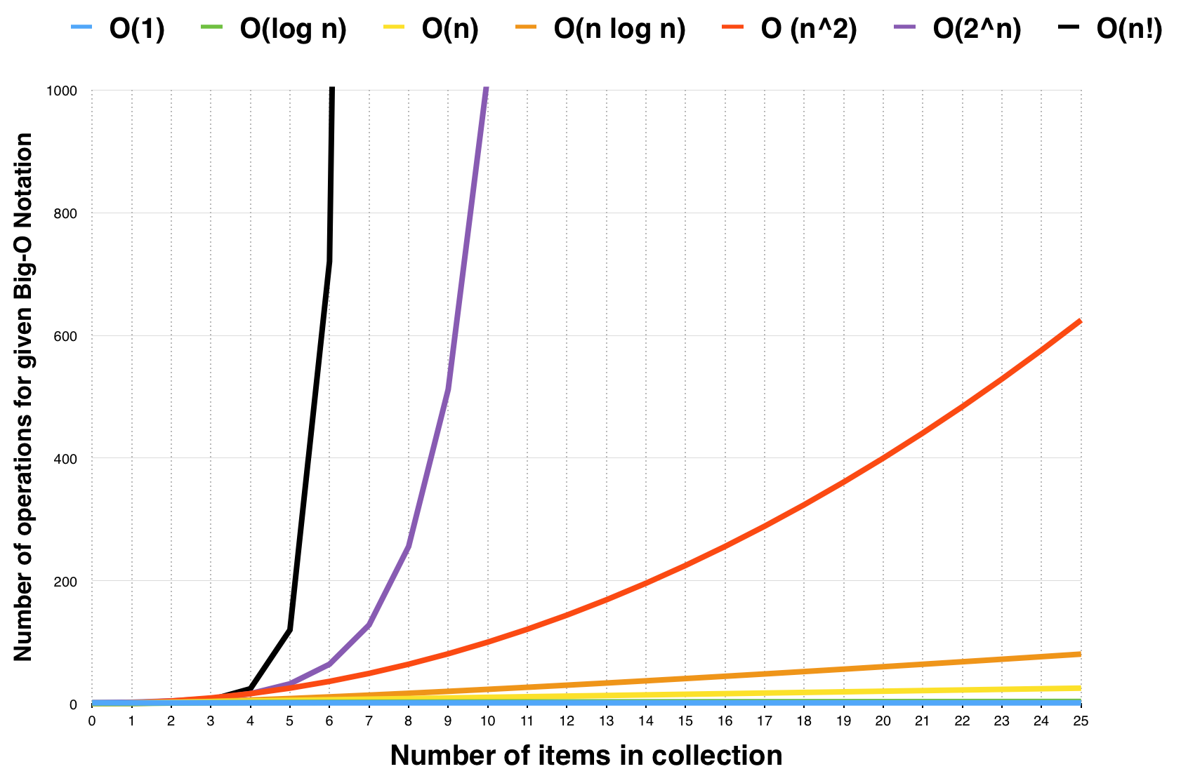
We will now look into some of the most common complexities.

Constant Time or Ο(1)

This is when the algorithm runs in constant time ,i.e, doesn't depend on the size of the input. For example,

int start = 10;
int end = 20;
int mid;
mid = (start + end)/2;

Linear Time or Ο(N)

This is when the runtime of the algorithm grows linearly with the size of the input. For example,

for(int i=0;i<n;i++)
    cout << i << endl;

Quadratic Time or Ο(N²)

This is when the runtime of the algorithm grows quadratically with respect to the size of the input. For example,

for(int i=0;i<n;i++)
{
    for(int j=0;j<n;j++)
        cout << i+j << endl;
}

Logarithmic Time or Ο(log N)

This is when the algorithm breaks down into two subproblems. For example, the binary search algorithm follows Ο(log N) complexity.

int binsearch(int arr[],int low,int high)
{
    int mid = (low + high)/2;
    if(item == arr[mid])
        return mid;
    if(item > arr[mid])
        return binsearch(arr,mid+1,high);
    return binsearch(arr,low,mid-1);
}

The logarithm is base 2, i.e, log₂N

Comparison between standard complexities

---

Further Reading

1. Chapter 1,3 of Introduction to Algorithms, Second Edition, by Thomas Cormen, Charles Leiserson, Ronald Rivest, Clifford Stein.
2. https://www.topcoder.com/community/data-science/data-science-tutorials/computational-complexity-section-1/
3. https://www.cs.cmu.edu/~adamchik/15-121/lectures/Algorithmic%20Complexity/complexity.html
4. https://www.hackerearth.com/practice/basic-programming/complexity-analysis/time-and-space-complexity/tutorial/
5. http://bigocheatsheet.com/ - contains complexities of standard sorting algorithms and standard data structures