3_visualization
For more details of the commands, use -h option to see the usage.
LiCSBAS_disp_img.py -i image_file -p par_file [-c cmap] [--cmin float]
  [--cmax float] [--auto_crange float] [--n_color int] [--cycle float]
  [--nodata float] [--bigendian] [--png pngname] [--kmz kmzname]

 -i  Input image file in float32, uint8, GeoTIFF, or NetCDF
 -p  Parameter file containing width and length (e.g., EQA.dem_par or mli.par)
     (Not required if input is GeoTIFF or NetCDF)
 -c  Colormap name (Default: SCM.roma_r, reverse of SCM.roma)
     Available colormaps (all cmap can be reversed with "_r"):
     - Matplotlib predefined name (e.g. viridis)
       https://matplotlib.org/tutorials/colors/colormaps.html
     - Scientific colour maps (e.g. SCM.roma)
       http://www.fabiocrameri.ch/colourmaps.php
     - Generic Mapping Tools (e.g. GMT.polar)
       https://docs.generic-mapping-tools.org/dev/cookbook/cpts.html
     - cmocean (e.g. cmocean.phase)
       https://matplotlib.org/cmocean/
     - colorcet (e.g. colorcet.CET_C1)
       https://colorcet.holoviz.org/
     - cm_insar (GAMMA standard rainbow color for wrapped phase)
     - cm_isce (ISCE standard rainbow color for wrapped phase)
 --cmin|cmax    Min|max values of color (Default: None (auto))
 --auto_crange  % of color range used for automatic determination (Default: 99)
 --n_color    Number of rgb quantization levels (Default: 256)
 --cycle        Value*2pi/cycle only if cyclic cmap (i.e., insar or SCM.*O*)
                (Default: 3 (6pi/cycle))
 --nodata       Nodata value (only for float32) (Default: 0)
 --bigendian    If input file is in big endian
 --png          Save png (pdf etc also available) instead of displaying
 --kmz          Save kmz (need EQA.dem_par for -p option)
This script displays an image file.

LiCSBAS_plot_ts.py [-i cum[_filt].h5] [--i2 cum*.h5] [-m yyyymmdd] [-d results_dir]
    [-u U.geo] [-r x1:x2/y1:y2] [--ref_geo lon1/lon2/lat1/lat2] [-p x/y]
    [--p_geo lon/lat] [-c cmap] [--nomask] [--vmin float] [--vmax float]
    [--auto_crange float] [--dmin float] [--dmax float] [--ylen float]
    [--ts_png pngfile]

 -i    Input cum hdf5 file (Default: ./cum_filt.h5 or ./cum.h5)
 --i2  Input 2nd cum hdf5 file
       (Default: cum.h5 if -i cum_filt.h5, otherwise none)
 -m    Refereference (master) date for time series (Default: first date)
 -d    Directory containing noise indices (e.g., mask, coh_avg, etc.)
       (Default: "results" at the same dir as cum[_filt].h5)
 -u    Input U.geo file to show incidence angle (Default: ../GEOCml*/U.geo)
 -r    Initial reference area (Default: same as info/*ref.txt)
       0 for x2/y2 means all. (i.e., 0:0/0:0 means whole area).
 --ref_geo   Initial reference area in geographical coordinates.
 -p    Initial selected point for time series plot (Default: ref point)
 --p_geo     Initial selected point in geographical coordinates.
 -c    Color map for velocity and cumulative displacement.
       See help of LiCSBAS_disp_img.py.
       (Default: SCM.roma_r, reverse of SCM.roma)
 --nomask     Not use mask (Default: use mask)
 --vmin|vmax  Min|max values of color for velocity map (Default: auto)
 --dmin|dmax  Min|max values of color for cumulative displacement map
              (Default: auto)
 --auto_crange  Percentage of color range used for automatic determination
              (Default: 99 %)
 --ylen       Y Length of time series plot in mm (Default: auto)
 --ts_png     Output png file of time series plot (not display interactive viewers)
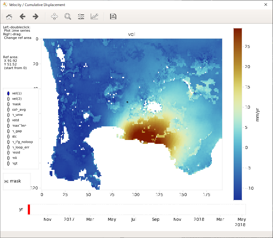
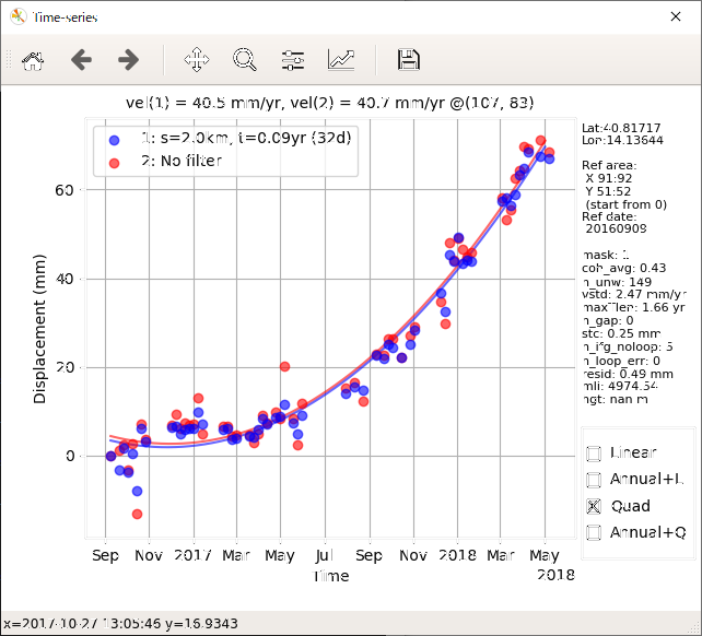
This script displays the velocity, cumulative displacement, and noise indices, and plots the time series of displacement. You can interactively change the displayed image/area and select a point for the time series plot. The reference area can also be changed by right dragging.
Demonstration Video (High resolution mp4, 20MB)
LiCSBAS_profile.py -i infile -p dempar [-r x1,y1/x2,y2] [-g lon1,lat1/lon2,lat2] [-o outfile] [--bigendian] [--nodisplay]

 -i  Input file (float, little endian)
 -p  Dem parameter file (EQA.dem_par)
 -r  Point locations in xy coordinates
 -g  Point locations in geographical coordinates
 -o  Output text file (Default: profile.txt)
     Format: lat lon x y distance value (x/y start from 0)
 --bigendian  If input file is in big endian
 --nodisplay  Not display quick look images

 Note: either -r or -g must be specified.
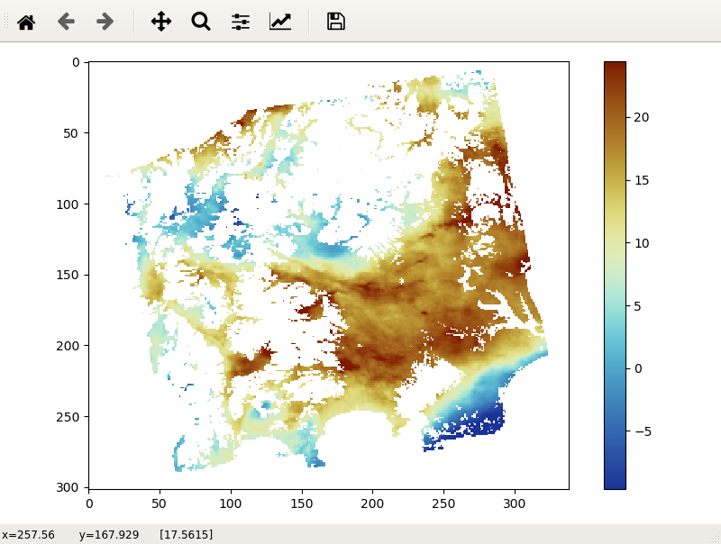
This script gets a profile data between two points specified in geographical coordinates or xy coordinates from a float file. A quick look image is displayed and a text file and kml file are output.

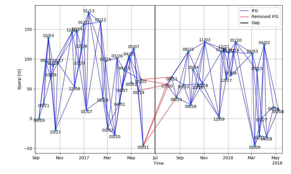
LiCSBAS_plot_network.py -i ifg_list -b bperp_list [-o outpngfile] [-r bad_ifg_list] [--not_plot_bad]

 -i  Text file of ifg list (format: yyymmdd_yyyymmdd)
 -b  Text file of bperp list (format: yyyymmdd yyyymmdd bperp dt)
 -o  Output image file (Default: netowrk.png)
     Available file formats: png, ps, pdf, or svg
     (see manual for matplotlib.pyplot.savefig)
 -r  Text file of bad ifg list to be plotted with red lines (format: yyymmdd_yyyymmdd)
 --not_plot_bad  Not plot bad ifgs with red lines
This script creates a png file (or in other formats) of SB network. A Gap of the network are denoted by a black vertical line if a gap exist. Bad ifgs can be denoted by red lines.
LiCSBAS_color_geotiff2tiles.py -i infile [-o outdir] [--zmin int] [--zmax int]
 [--xyz] [--n_para int]

 -i  Input color GeoTIFF file
 -o  Output directory containing XYZ tiles
     (Default: tiles_[infile%.tif], '.' will be replaced with '_')
 --zmin  Minimum zoom level to render (Default: 5)
 --zmax  Maximum zoom level to render (Default: auto, see below)
         17 (pixel spacing <=   5m)
         16 (pixel spacing <=  10m)
         15 (pixel spacing <=  20m)
         14 (pixel spacing <=  40m)
         13 (pixel spacing <=  80m)
         12 (pixel spacing <= 160m)
         11 (pixel spacing >  160m)
 --xyz     Output XYZ tiles instead of TMS (opposite Y)
 --n_para  Number of parallel processing (Default: # of usable CPU)
           Available only in gdal>=2.3
This script generates directory with TMS tiles using gdal2tiles.py.
Prototype code available here, thanks to Dr. Milan Lazecký.
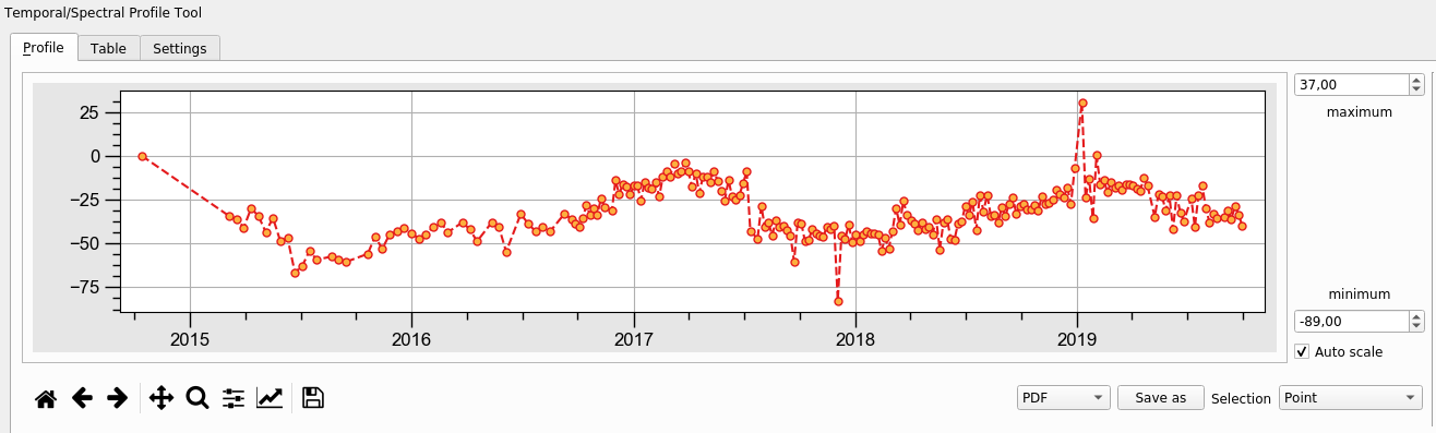
This script outputs a standard NetCDF4 file using LiCSBAS results, which can be directly read by QGIS. Modules xarray and rioxarray are required. A QGIS plugin "Temporal/Spectral Profile Tool" can plot the time series at an selected point.