Home

What is Hypertime ?

The Wrapped Hypertime (WHyTe) is an enabling technology for long-term mobile robot autonomy in changing environments [1], but is applicable to problems outside the robotics domain. It allows to introduce the notion of dynamics into most spatial models used in the mobile robotics domain, improving ability of robots to cope with naturally-occuring environment changes. Hypertime is based on an assumption that from a mid- to long-term perspective, some of the environment dynamics are periodic. To reflect that, Hypertime models extend spatial models with a set of wrapped time dimensions that represent the periodicities of the observed variations. By performing clustering over this extended representation, the obtained model allows the prediction of probabilistic distributions of future states and events in both discrete and continuous spatial representations.

The idea builds on the success of the Frequency Map Enhancement (FreMEn), which also models periodic changes and was shown to improve efficiency of mobile robots as they learned the dynamics of their operational environments.

What is the core idea ?

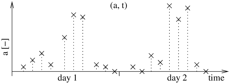
Let's say that you measured the number of people present in a certain area and you want to use the learned data to predict how many people will be present in the future. Hypertime takes the data points (a,t) observed over time (top, black) and processes them by frequency analysis~FreMEn to determine a dominant periodicity T. Then, it projects the time t onto a 2d space (called hypertime) and the vectors (a,t) become _(a, cos(2π t/T), sin(2π t/T))$ (bottom, left). The projected data are then clustered (bottom, center, blue) to estimate the distribution of a over the hypertime space (green). Projection of the distribution back to the uni-dimensional time domain allows to calculate the probabilistic distribution of a for any past or future time.

Any detailed explanation ?

Let us explain using the same example again: Let's say that you measured the number of people present in a certain area. Let's say that every time t_i you do the measurement, you obtain a number a_i. After two days of measurements, you will get data that might look like the ones in Figure 1.

Now say that you want to predict the number of people for day 3 at 5pm. Ideally, you would like to have some model, that could tell you how likely it is to measure a given a at a given time t. In other words, you want to have a way to obtain a conditional probability density function p(a|t). The method presented here provides such a model by processing the data as follows:

Initialisation

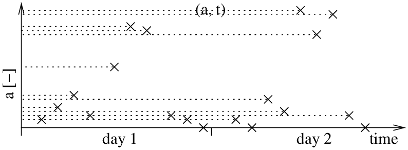
First, we store all measurements a_i as ⁰x_i. This means that we neglect the time domain for now and we only consider the values of a, which corresponds to the vertical axis of the graph, see Figure 2.

Iteration 0

Clustering

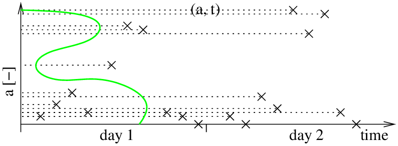
To obtain p(a), we run clustering over the ⁰x_i. Let's say that we chose to use Gaussian mixtures with two clusters. We should get an estimate of the probabilistic distribution of a as displayed in green in Figure 3. After this step, we can estimate the probability of obtaining a given measurement a. Although we could estimate the probabilistic distribution of a analytically, a practical solution to estimate it is calculating p(a) over the domain of a in a numerical way.

Model Error Estimation

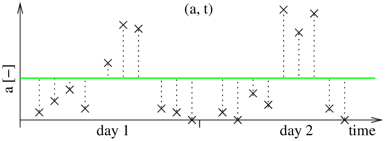
Using the model from the previous step, we predict the value of a'_i for every time t_i and we calculate an error _e_i=_a'_i-_a_i. We sum the square of all the errors, obtaining the model error ⁰E. Since our model neglects time, the predicted values for all _a_i will be identical and equal to the mean of the GMM model build in the previous step. The errors we get will look like this:

Identification of periodicities

Now, we take the errors _e_i and times _i_i we check if they exhibit any periodical pattern. In practice, we use the FreMEn tool, based on the Fourier Transform to find if there is any periodicity. The Fourier Transform will tell us that the error exhibits a strong daily periodicity T₁. This basically corresponds to finding the best sine wave to fit the errors.

Hypertime space extension

Now, we take all values in ⁰x_i and add the temporal information to them. This is done by extending each ⁰x_i with two additional values sin( 2π t_i /T₁ ) and cos( 2π t_i /T₁ ), obtaining a vector ¹x_i = ( a_i, sin( 2π t_i /T₁ ), cos( 2π t_i /T₁ ) ). This causes the original timeline of a_i on Figure 1 to wrap around a unit circle, forming a cylinder as shown in Figure 3. In this space, measurements a_i from the similar time of the day will get close to each other, and form natural clusters characterising the number of people around at a given time of the day. Once the points are projected, we start with the next iteration.

Iteration 1

Clustering

This time, we run clustering over the ¹x_i. Let's say that we chose to use Gaussian mixtures with three clusters, and we can obtain clusters as on Figure 4. This model allows us to calculate the joint probability p(a,t) be projecting it into the hypertime space, i.e. to ( a, sin( 2π t/T₁), cos( 2π t/T₁) ) and calculating the membership function of the projected point to the aforementioned clusters.

Model Error Estimation

Knowledge of the p(a,t) allows to determine the most likely a for a given time t. Thus, we calculate the training set datapoints errors e_i and overall model error ¹E as during the first iteration.

Identification of periodicities

Again, we use the FreMen to extract a dominant periodicity in the error e_i, obtaining a second periodicity T₁. However, the value of T₂ is unlikely to reflect real periodicity in the data.

Hypertime space extension

Again we extend every ¹x_i with two additional values sin( 2π t_i /T₂ ) and cos( 2π t_i /T₂ ), obtaining a set of vectors ²x_i = ( a_i, sin( 2π t_i /T₁ ), cos( 2π t_i /T₁ ), sin( 2π t_i /T₂ ), cos( 2π t_i /T₂ ) ). Then, we proceed with a next iteration.

Iteration 2

Clustering

This time, we run clustering over the ²x_i obtaining a model capable to represent p(a,t) through projection of (a,t) into a 5D space from the previous step.

Model Error Estimation

Knowledge of the p(a,t) allows to determine the most likely a for a given time t. Thus, we calculate the training set datapoint errors e_i and overall model error ²E as during the first iteration. Since T₂ is unlikely to represent a real periodicity, the model error ²E will be higher than the error ¹E calculated during iteration 1. Thus, we will terminate the algorithm and use the model constructed during the clustering stage of iteration 1.

How to make predictions

The model that we obtained calculates the joint probability p(a,t) by projecting _(a,t)) into ( a, sin( 2π t/T₁), cos( 2π t/T₁) ) and calculating its membership function to the clusters formed in the clustering step. However, prediction for a given time means that you want to calculate the conditional probability p(a|t). To do so, we first estimate the conditional probabilistic distribution p(a|t) over the domain of a. This is performed in a practical manner - we fix the time t, for which we want to perform a prediction and we choose the values of a_c, which represent a's domain with sufficient granularity. Then, we project these values into the hypertime space, i.e. we form ( a_c, sin( 2π t/T), cos( 2π t/T) ) and calculate _p(a_c,t) = p( a_c, sin( 2π t/T), cos( 2π t/T) ) for all values of a_c. Then, we normalize the results so that the sum of p(a_c,t) over all a_c's is 1.

For details, please refer to the papers published so far:

References

1. T.Krajnik, T.Vintr, S.Molina, J.P.Fentanes, G.Cielniak, T.Duckett: Warped Hypertime Representations for Long-term Autonomy of Mobile Robots Arxiv, 2018. [bibtex]

2. T.Vintr, Z.Yan, T.Duckett, T.Krajník: Spatio-temporal representation for long-term anticipation of human presence in service robotics. In proceedings of the IEEE International Conference on Robotics and Automation (ICRA), 2019. [bibtex]