design
The R GBM package allows users to train gradient boosting machines primarily for the purposes of prediction and feature selection. The package is built using RCpp and is composed of two parts: a R front-end that takes user inputs and performs pre-processing before passing a series of arguments to the second part; the C++ back-end. The main algorithmic work is done in the C++ layer, which on completion passes R objects back to the R front-end for postprocessing and reporting. This design document focusses on the C++ back-end, providing descriptions of its scope, functionality and structure; for documentation on the R API please see the R GBM package vignettes.
The C++ back-end, from here on referred to as the "system", provides algorithms to: train a GBM model, make predictions on new data using such a fitted model and calculate the marginal effects of variable data within such a fitted model via "integrating out" the other variables. The main bulk of the C++ codebase focusses on the training of a GBM model, tasks involved in this process include: set-up of datasets, calculation of model residuals, fitting a tree to said residuals and determining the optimal node predictions for the fitted tree. The other pieces of functionality, that is prediction and calculating the marginal effects of variables, are singular functions with little or no developer designed classes associated with them.
The structure imposed on the C++ back-end was selected to:
-
Replace a legacy setup with one more amenable to change.
-
Make the structure and functionality of the system more transparent via appropriate OO design and encapsulation.
-
Implement design patterns where appropriate - in particular to simplify memory management through the application of the RAII idiom.
Within the GBM package the system performs the main algorithmic calculations. It undertakes all of the algorithmic work in training a gradient boosted model, making prediction based on new covariate datasets and calculating the marginal effects of covariates given a fitted model. It does not perform any formatting or postprocessing beyond converting the fitted trees, errors etc. to a R list object and passing it back to the front-end.
Due to the algorithmic nature of the system, the description of the system
will focus on the behaviour of the system and its structure is
captured by the Functional and Development views respectively. Within
the package the system is located in the /src directory. To
conclude this introduction, it should be noted that the system has
been developed in line with Google C++ style.
The main use cases of the system are:
- Training a gradient boosted model using data and an appropriate statistical model.
- Predicting the response from new covariates using a trained model.
- Calculating Marginal effects of data using a trained model.
The system is composed of numerous classes used almost exclusively for
training along with an interface to the R front-end. This entry point
is appropriately named gbmentry.cpp and contains 3 functions: gbm,
gbm_pred and gbm_plot. These functions perform the training,
prediction and marginal effects calculations described in the previous Section
respectively. The functionality and dynamic behaviour of these
methods will now be described.
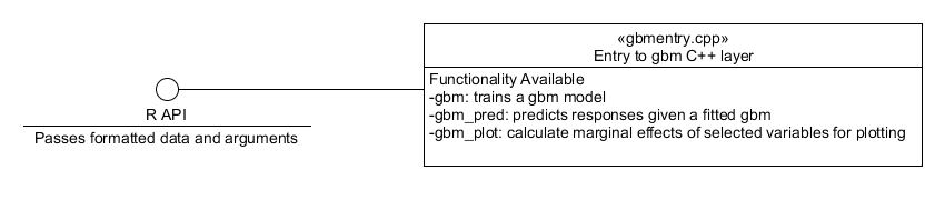 Figure 1. Component diagram showing the interface between the R layer and the system.
The procedure to train a gbm model follows a sequence of simple steps
as shown in Figure 2. Upon entry to the gbm method the user specified
parameters are converted to an appropriate GBM configuration objects,
see datadistparams.h and treeparams.h. These configuration
objects are then used to initialize the GBM engine, this component
stores both the tree parameters, which define the tree to be fitted,
and the data/distribution container. Upon initialization the GBM
engine will also initialize an instance of an appropriate dataset
class, a bagged data class and a distribution object from the GBM
configuration object. The dataset object contains both the training
and validation data; these sets live together in vector containers and
to swap between them the pointer to the first element in the set of
interest is shifted by the appropriate amount. The bagged data class
defines which elements of the dataset are used in growing an
individual tree; how these elements are chosen is distribution
dependent. After this, the GbmFit object is initialized. This object
contains the current fitted learner, the errors associated with the
fit and the function estimate (a Rcpp numeric vector). The function
estimate is set to the previous estimates if provided or an
appropriate value for the distribution selected otherwise.
With the GBM engine and the fit object initialized, the algorithm loops over the number of trees to fit and performs the following actions:
- Create a tree object.
- Bag the data to use for fitting the tree.
- Calculate the residuals using the current estimate, bagged data and distribution object.
- Fit the tree to the calculated residuals - this is done by generating all possible splits for a subset of variables and choosing the split to minimize the variance of the residuals within nodes. The best splits for each node are cached so if a node is not split on this round, no future splitting of that node is evaluated.
- Set the terminal node predictions which minimize the error.
- Adjust the tree, so non-terminal nodes also have predictions.
- Update the estimate, for both training and validation sets, and calculate the: training errors, validation errors and the improvement in the out of bag error from the update.
- Wrap up the fitted tree and errors, along with a reference to the dataset, in a FittedLearner object (see
FittedLearner.h).
The returned fitted learner object defines the "current fit" in the
GbmFit object, which is used to update the errors. At the end of a
single iteration, the tree and the associated errors are converted to
a R List representation which is then output to the R layer once all
the trees have been fitted.
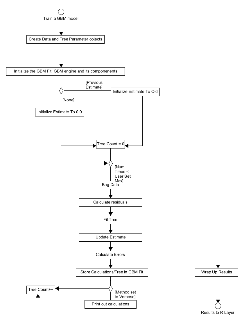 Figure 2. Activity diagram for the process of training a GBM model.
The bagging of the data from the training set and calculation of residuals is distribution dependent and so is incorporated in the system as appropriate methods in the distribution class and its container. The tree object is comprised of several components, the principle ones are: a root node, a vector of the terminal nodes and a vector mapping the bagged data to terminal nodes. A node splitter which generates and assigns the best potential split to each terminal node is used in the tree growing method. This structure is shown below in Figure 3.
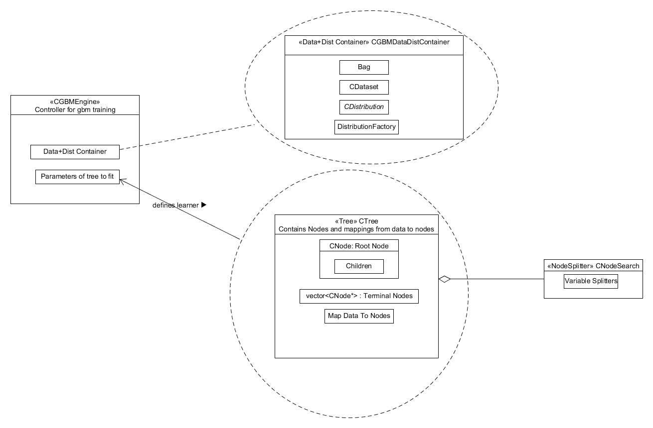 Figure 3. Component diagram showing what the GBM Engine component is comprised of.
Using a previously fitted GBM model, the system can predict the
response of further covariate data. The R frontend passes the
following variables to the gbm_pred function in gbmentry.cpp: the
covariates for prediction, the number of trees to use to predict, the
initial prediction estimate, the fitted trees, the categories of the
splits, the variable types and a bool indicating whether to return the
results using a single fitted tree or not.
The prediction for the new covariates is then initialized, either to the previous tree prediction or the initial estimate value from the model training if it is the first tree prediction to be calculating. The number of trees to be fitted is then looped over, within each iteration the observations are in the covariate dataset are also looped over. Each observation is initially in the root node, a counter which tracks the current node the observation is in is thus set to 0. This observation is then moved through the tree, updating its current node, until it reaches the appropriate terminal node. Once the algorithm reaches a terminal node, the prediction for that observation and tree is set to the final split value of the terminal node's parent in the tree. This process is repeated over all observations and for all trees, once completed the prediction vector is wrapped up and passed back to the R front-end, see Figure 4.
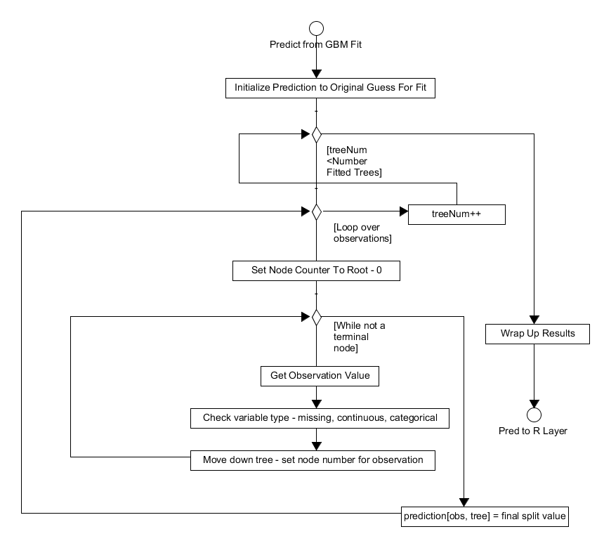 Figure 4. Activity diagram showing how the algorithm performs predictions on new covariate data.
The final piece of functionality offered by the system is to calculate
the marginal effects of a variable by "integrating" out the others. As
well as a fitted gbm model and covariate data the user also specifies which
variables they're interested in at the R layer. This method utilises a
NodeStack class which is defined at the beginning of gbmentry.cpp,
this is a simple class that defines a stack of pairs. These pairs contain
the node index, that is what node in the tree we are looking at, and its
weight.
With this in mind the method works as follows:
- the initial prediction is set to user specified initial values.
- the algorithm loops over the number of trees to fit.
- the algorithm then loops over the observations.
- in the observation loop it creates a root node, puts it on the stack and sets the observation's current node to be 0 with weight 1.0.
- it gets the top node off the stack and checks if it is split.
- (a) if it isn't split the predicted function for this variable and tree is set to the split value times the weight of the node.
- (b) if the node is non-terminal it checks if the split variable is in the user specified variables of interested. If so the observation is moved to the appropriate child node which is then added to the stack. If this is not the case, two nodes (an average of both left/right splits - this "integrates" out the other variables) are added to the stack and it returns to step 5.
- When the observation reaches a terminal node it gets another observation and repeats steps 5 & 6.
- With all trees fitted the predicted function is wrapped up and output.
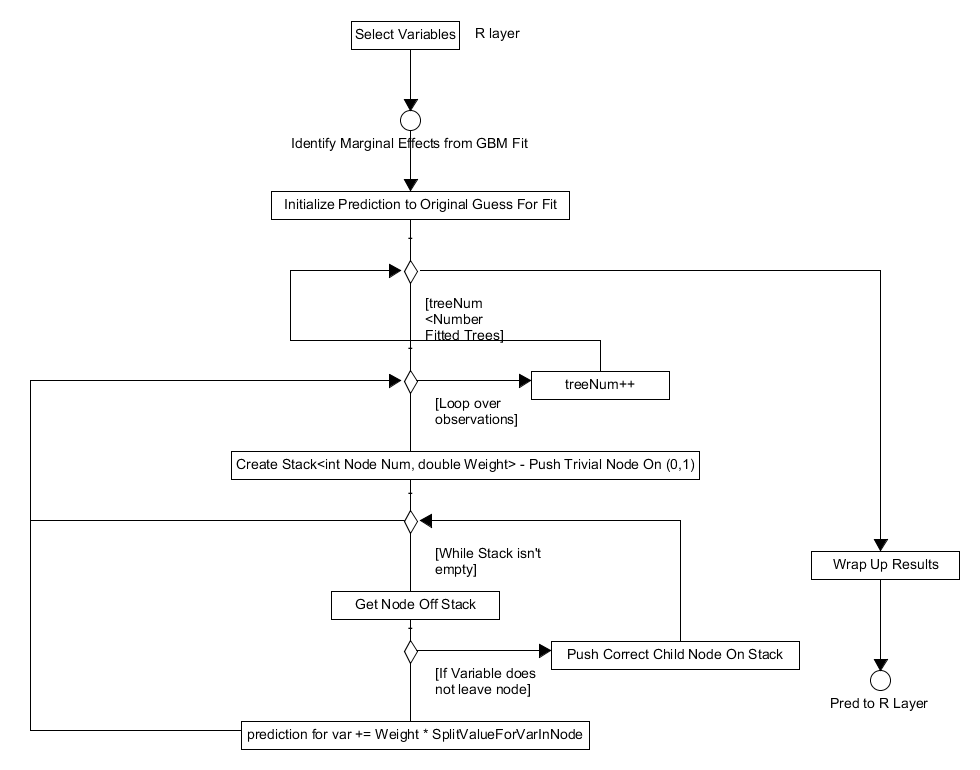 Figure 5. Activity diagram for calculating the marginal effects of specific variables.
The near entirety of the system is devoted to the task of training a
gbm model and so this Section will focus on describing the classes and
design patterns implemented to meet this end. Starting at a high
level the primary objects are the "gbm engine" found in
gbm_engine.cpp and the fit defined in gbm_fit.h. The component
has the data and distribution container, see gbm_datacontainer.cpp,
and a reference to the tree parameters (treeparams.h) as private
members; this is shown in Figure 3. The "gbm engine" generates the
initial function estimate and through the FitLearner method which
run the methods of the gbm_datacontainer.cpp and tree.cpp to
perform tasks such as growing trees and calculating errors/bagging
data. The system is built on the RAII idiom and these container
classes are initialized on contruction of this gbm engine object and
released on its destruction. This idiom is applied across the system
to simplify the task of memory management and further elicit
appropriate object design. Beyond this, encapsulation and
const. correctness are implemented where possible within the system.
The R layer passes a number of parameters/R objects to the system.
These are converted to appropriate parameters and stored in simple
objects for use in initializing the data and distribution container
and tree objects. After construction of the gbm engine the
DataDistParams class is not used again during training while the
TreeParams object are stored within the engine and used to
initialize trees for fitting on each iteration.
The dataset class, dataset.h, is part of the data/distribution container
and is initialized using the DataDistParams described in the previous
Section. This class stores both appropriate R objects, e. g. the response
is stored as RCpp::NumericMatrix, and standard C++ datatypes describing
the data, e. g. unsigned long num_traindata_. To iterate over these R
vectors/arrays the dataset object has appropriate pointers to these arrays
which can be accessed via the corresponding getter methods. The R objects
stored here contain both training and validation data, to access a particular
dataset the appropriate pointers are shifted by the length of the dataset
so they point to the beginning of the validation/training set. Most of this
class is defined within the header as the number of calls to the dataset's
getter functions means that inlining these methods has a significant impact
on the system's overall performance. It also has a RandomOrder() method
which takes the predictor variables and shuffles them, this is used during
the tree growing phase where all splits are generated for a random subset
of features in the data. Finally, an associated class is the "Bag"; this
class contains a vector of integers (0/1's) called the "bag" which defines
the training data to be used in growing the tree.
The distribution class, distribution.h, is an abstract class which
defines the implementation any other distributions to be included in
the system must follow. The distribution object performs numerous
features using an instance of thedataset class defined in the previous
Section. Importantly it constructs the bag for the data, this method
appropriately titled BagData is only different for the pairwise
distribution where data groupings affect the bagging procedure.
Before constructing the bags, the distribution object needs to be
initialized with the data. This initialization will take the data
rows and construct a multi-map which maps those rows to their
corresponding observation ids, often each row is an unique observation
but this is not always the case. This multi-map ensures bagging occurs
on a by-observation basis as opposed to a by-row basis, as the latter
would result in overly optimistic errors and potentially a failure of
the training method where data from a single observation could appear
both in the bag and out of it. The distribution object is also
responsible for calculating the residuals for tree growing, the errors
in the training and validation sets, initializing the function
estimate and calculating the out of bag error improvement on fitting a
new tree. These methods are all accessed via its container class
stored within the gbm engine object.
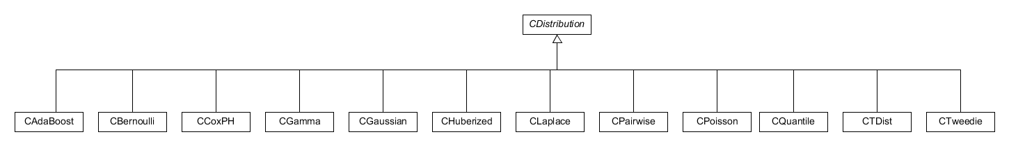 Figure 6. Diagram showing the distributions currently implemented within the system.
The construction of the a distribution object is done using a dynamic
factory pattern, see Figure 7. In this design, the constructors of
the concrete distribution classes are private and they contain a
static Create method. This method is registered to a map in the
factory, distribution_factory.cpp, where the name of the
distribution, a string, is its key. On creation of a gbm engine
object, a distribution factory is created and the appropriate
distribution is generated from the factory using the user selected
distribution, a string which acts as key to the same map, and
DataDistParams struct.
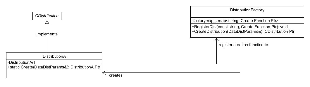 Figure 7. Dynamic Factory pattern used to control the creation of distribution objects. The distribution factory itself is a singleton.
To conclude this subsection, there are some concrete distribution
specific details to describe. The pairwise distribution,
CPairwise.h, uses several objects which specify the information
ratio measure that this distribution uses in its implementation.
These classes all inherit from an abstract IRMeasure class and are
defined in the CPairwise.h and CPairwise.cpp files.
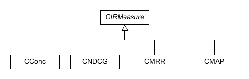 Figure 8. Diagram displaying the information ratio classes used by the pairwise distribution.
The other distribution which has a unique design is the Cox partial
hazards model. The Cox partial hazards model is a survival model
whose implementation depends on whether the response matrix provided
to the system is that of "censored" data or "start-stop" data. In
essence, if the response matrix has 2 columns it is censored and if it
has more than 2 it is start-stop. To incorporate this added
complexity, the CCoxPH.h class follows a state pattern, whereby the
Cox PH object contains a pointer to an object implementing the correct
methods for a specific scenario and those objects contain a pointer to
the Cox PH object. This design is shown in Figure 9.
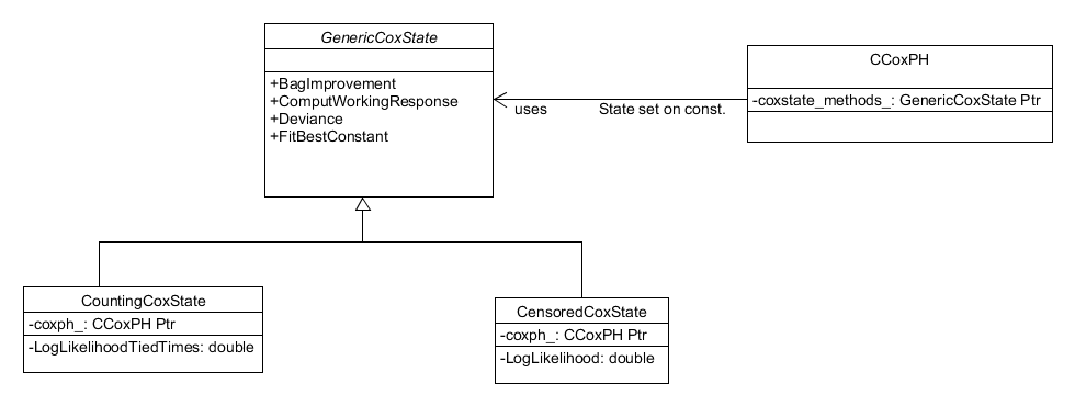 Figure 9. The Cox Partial Hazards distribution employs a state design pattern to accommodate the dependency of its implementation on the response matrix.
The final component of the gbm engine to consider is the tree class
defined in tree.h. As described in "Training a GBM model" subsection the tree class
contains: a rootnode, of class CNode, a vector of pointers to
terminal nodes, a vector assigning data to those terminal nodes, a
node search object (see node_searcher.h) and various data describing
the tree (such as its maximum depth etc.). The tree class has methods
that grow the tree, reset it for another growth, prediction on
validation data, adjusting the tree once predictions are assigned to
the terminal nodes and outputting it in a suitable format for the R
layer to use.
The most important part of this class is the method for the growing of
the tree. A key component in growing a tree is identifying appropriate
splits, this role is the responsibility of the node searcher
object. The node searcher object stores the best split identified for
each terminal node. It uses vectors of variable splitters (see
vec_varsplitters.h and varsplitter.h) to determine the best splits
generated for each node and for each variable. Within the
GenerateAllSplits() method, one vector of NodeParams, see below,
copies the current best splits stored in the node searcher object.
The variables to split on are then looped over and a vector of
variable splits, one for each terminal node, is initialized to
calculate the best split for the current variable in each node. The
best split for the current variable is extracted from this vector and
used to update the copy of the best splits. At the end of this loop,
the updated copy of best splits are then assigned to the best splits
stored in the node search object. This design follows a MapReduce
structure and allows for parallelisation of this search process; the
details of this parallelisation (see parallel_details.h) are also
stored as a private member in the node search class.
The node class itself contains pointers to its children and its
methods, such as calculating predictions, are dependent on the type of
split present. The node can either be terminal, so it has no split,
or have a continuous/categorical split. To account for this
dependency on the split, the node class is implemented with a state
design pattern , similar to the Cox PH distribution, but in this
instance it posseses a SetStrategy() method so the implementation of
a node can change as a tree grows. The variable splitter objects
contain "node parameters", see node_parameters.h, which encapsulate
the properties of the proposed split nodes. These NodeParams
objects use NodeDef structs, located in node_parameters.h, to
define the proposed node splits and provides methods to evaluate the
quality of the proposed splits. Finally, the varsplitter class has a
state design pattern where on construction the methods for how the
variable of interest should be split are set, see Figure 11.
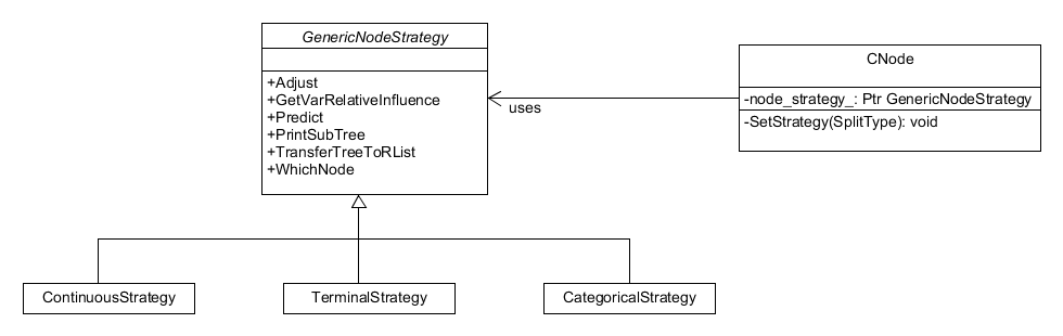 Figure 10. State pattern for the node object, it possesses a "SetStrategy()" method so nodes can change type as the tree grows.
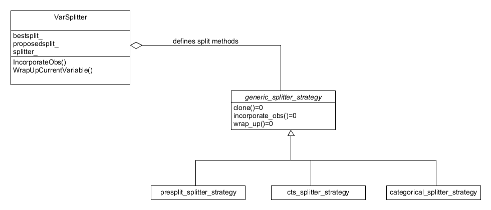 Figure 11. State pattern for the variable splitter object. How it splits on a variable is set on construction.
To conclude this Secion formal system class and interaction diagrams are presented in Figures 12 & 13 repsectively. These provide a complete and more detailed picture of the classes and their interactions which define the system, in particular the process of training a gbm.
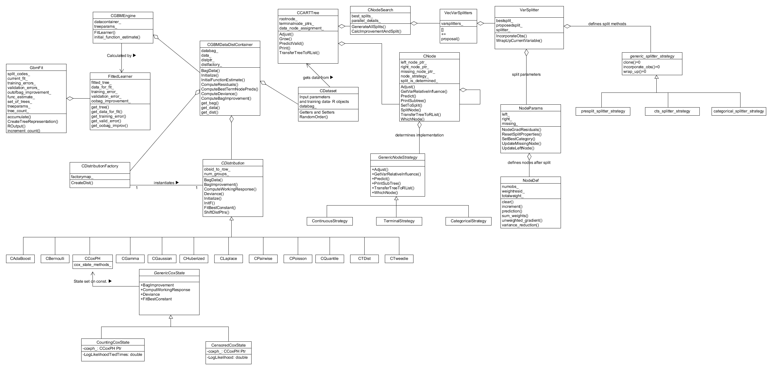 Figure 12. System class diagram showing the classes and how they interface in the training method.
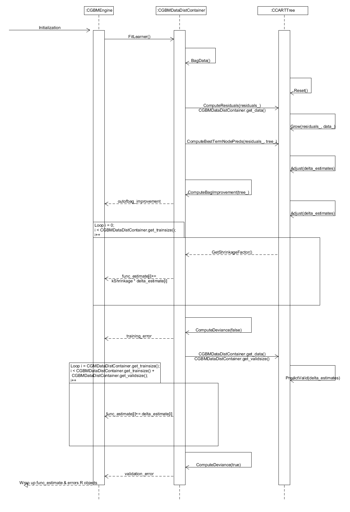 Figure 13. Sequence diagram for training a single tree when fitting a gradient boosted model.
The R GBM package consists of two parts: a R front-end that takes user inputs and pre-processes those inputs before passing a set of arguments to the second part, the C++ back-end, which does the main algorithmic calculations. The latter part of the package is described above; on completion of this calculation the results are passed back to the R layer for post-processing where it is wrapped into a model object and returned to the user for use in further calculations and reporting. This part of the wiki focusses on describing the R front-end, providing descriptions of its scope, functionality and structure - for further documentation on the R API and the functionality within, please see the R GBM package vignettes and in-built documentation.
The R front-end, which is referred to as the "system" for the remainder of this Section, provides an API that allows the user to: train a GBM model, make predictions on new data using a fitted mdoel, calculate and plot the marginal effects of variables on the model via "integrating out" the other variables as well as a whole host of other functionality such as additional fitting and ranking of the relative influence of variables within the boosted model. The primary purpose of the system is to take user inputs and pre-process them before calling the appropriate C++ functionality. The output from the back-end is then post-processed and the resulting output returned to the user for further manipulation and calculations. The primary task of fitting a GBM model has informed the design of the system and encompasses the most complex manipulations performed by the system. The other pieces of functionality provided by the system, are either purely functional in nature with no object orientated nature or rely upon the OO design tailored for the fitting a GBM model.
The structure imposed on the R front-end was selected to:
- Replace a legacy setup with one more amenable to change and maintenance.
- Make the functionality more modular and transparent via the use of appropriately design of S3 classes, methods and helper functions.
- Implement input checks where possible to constrain the behaviour of the system to be well-defined and explicit.
The system acts as the interface between the user and the algorithmic calculator which is the back-end. It provides an API to access the C++ back-end and performs all of the necessary pre-processing and post-processing associated with training a gradient boosted model, making predictions based on new predictor datasets and calculating the marginal effects of covariates within a fitted model. Beyond this, the system provides a suite of additional functionality including visualisations of the fitted models and trees, summaries of the fitted model object, model performance evaluation and calculation of the loss of the response given the predictions.
The description of the system will focus on the Functional and Development views respectively. This is due to the functional nature of the R programming language and the S3 OO system employed within the system. The system is located in the /R directory with the GBM package and was developed in line with the Hadley Wickham R Good Practice style.
The main use cases of the system that will be considered are:
- Pre-/Post-processing when training a gbm model using data and an appropriate statistical model.
- Processing for predicting responses from new covariates using a trained model.
- Evaluating the performance of a model.
- Pre- and post- processing associated with calculating the marginal effects.
The system is composed of a several classes which were created to elicit simple functionality and encapsulate data for the pre- and post-processing stages of model fitting. The main classes are as follows:
-
GBMDist- a distribution object which describes the model used in the algorithmic work. -
GBMTrainParams- an object capturing the user specified training parameters passed to the R API. -
GBMData- a data object constructed from the input data and model to enable manipulation of the data in preparation for model fitting or in other calculations. -
GBMVarCont- an object storing the properties of the predictor variables passed as arguments to the model fitting routine. -
GBMFit- a fitted gbm model.
The functionality and dynamic behaviour of the main use cases will now be described.
The user can train a gbm model through the functions gbmt and gbmt_fit, the former function is a general purpose
function that does some preprocessing before calling gbmt_fit, a more direct call to the C++ layer suitable for advanced users. The processes of these functions are shown in Figures 14. and 15. respectively. These functions take a number of arguments as inputs. In particular, the training parameters for fitting the model, e. g. the number of iterations, and the distribution are provided to the functions via GBMTrainParams and GBMDist objects respectively. These objects are created by calls to the training_params() and gbm_dist() constructors respectively, for more details on how this is done please see the vignettes within the package for details and examples. Upon entry into gbmt, the appropriate model parameters and predictor/response variables are extracted from the user inputs and the arguments checked to confirm their typing and validity. If possible the names of the predictor variables are extracted and stored to be passed later to gbmt_fit as an argument. The data provided may have specific groupings which have to be determined using the appropriately named S3 method - determine_groups. The training parameters are then updated accordingly to reflect any groupings within the data, specifically the number of training observations/groups to be used in the model fitting is updated, via the method update_num_train_groups(). After this update, the extracted model data and processed user inputs are passed to gbmt_fit.
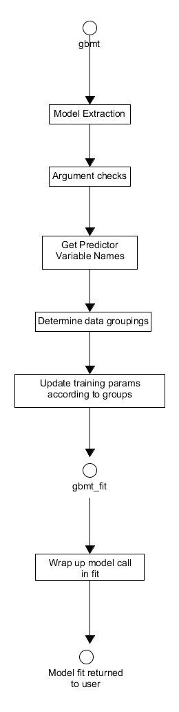 Figure 14. Activity diagram for the pre- and post-processing associated with training a gbm model using gbmt.
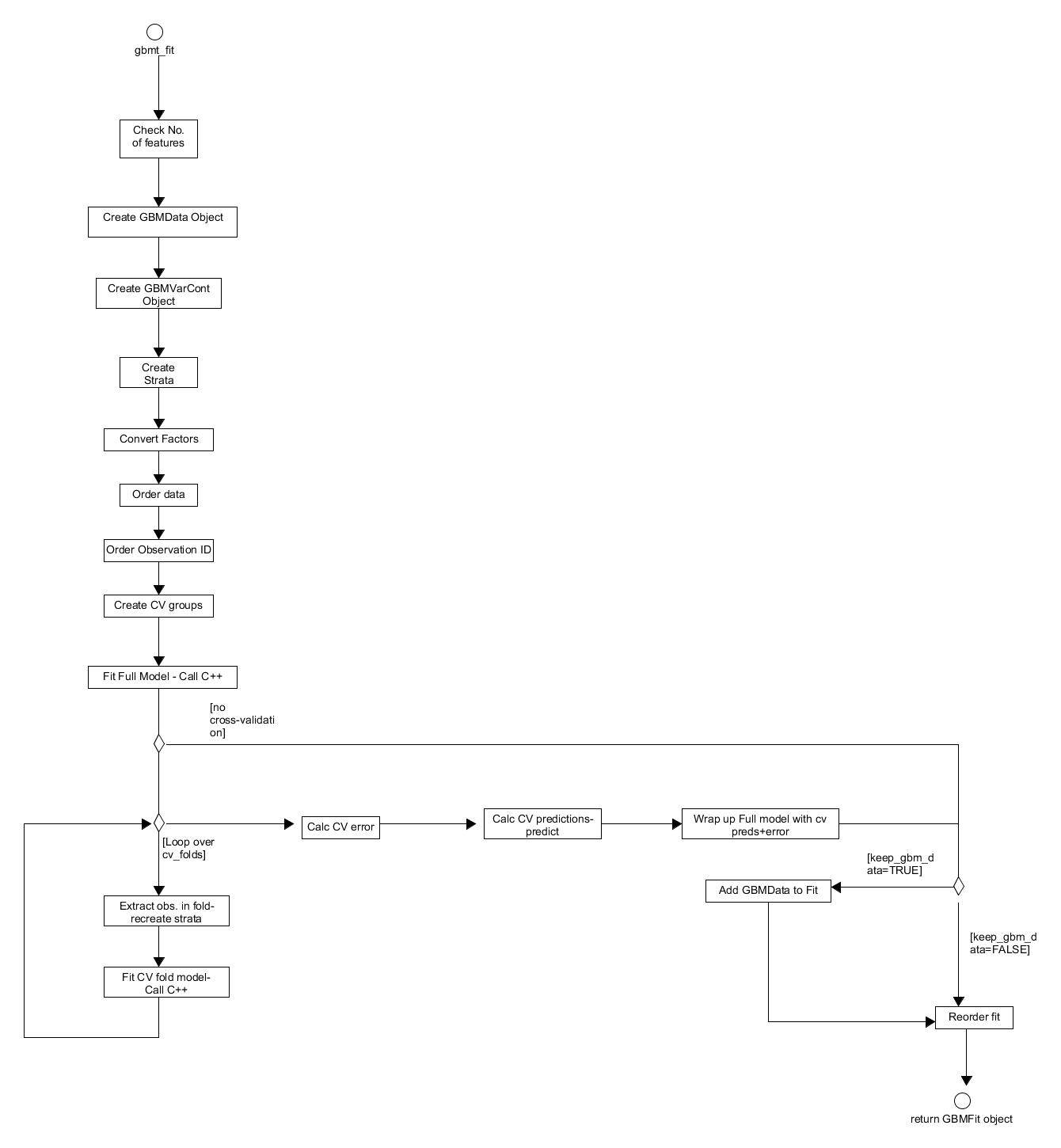 Figure 15. Activity diagram for training a gbm model through gbmt_fit.
The first step in the gbmt_fit process is to check the inputs, this is because it is directly accessible for advanced users and not just through gbmt; however, these checks do not overlap with those in gbmt. From the predictor and response data provided, a GBMData object is created via the constructor gbm_data(). The predictor variable properties, such as the monotonicity of their relationship with the output, are then passed to gbm_var_container to construct the appropriate GBMVarCont object which stores these properties. If the distribution object created defines a CoxPH model then the appropriate strata and sorting matrices are created and stored in the GBMDist object. The GBMData object then has its categorical factors converted to appropriate numerics, is ordered according to any groupings and the observation id and the order the predictor observations should be examined in when growing trees in the C++ layer is determined. The observation id are also appropriately ordered and cross-validation fold id are assigned to each observation via GBMDist S3 method - create_cv_groups.
With the pre-processing complete, a GBMFit model is built using all of the training data available with a call to the back-end. This object contains the GBMTrainParams, GBMDist and GBMVarCont objects used to train it as well as the outputs from the back-end algorithm such as the fitted trees. Afterwards, if the user specified that the model was to be cross-validated: a series of models are built where the training data is split into training folds and testing folds before updating the GBMDist and GBMTrainParams objects and calling the C++ layer (see gbm in the C++ design Section of the Wiki). The outputs of this process along with the full model are stored in a GBMCVFit object which is effectively a list of GBMFit objects. The cross-validation error and fits are then calculated. The latter is simply an average of the outcomes from calls to the predict method applied to each individual cross-validated GBMFit model. The full model is then augmented with these errors and predictions (along with parallelisation details) if they were calculated and the full GBMData object if the user specified. The full model fit is reordered, so it is in the appropriate order, before being passed back to caller.
Back at the gbmt layer, the full GBMFit model plus cross-validated data is further augmented with details of the model call before returning the fitted model object to the user.
Using a previously constructed GBMFit object, the system provides the user with an API to predict the response of additional
covariate data. This functionality is accessible through the S3 method predict which prepares the inputs before calling the C++ back-end to calculate the responses. The sequence of steps in this function is straightforward and displayed in Figure 16. Firstly, the user inputs are checked before the variable names are extracted from the fitted model, if those names are available, and applied to the new data. The named covariate data is then examined and any categorical data/factors are converted to appropriate numerics for the back-end. This function allows predictions from multiple iterations in the boosted fit can be calculated and so the next step is to ensure the requested iteration is within the scope of the fitted model. If a requested prediction iteration exceeds the number of previously fitted iterations the request is set to the maximum number of iterations used in constructing the boosted model. The requested iterations are then ordered before the back-end function gbm_pred is called to calculate the predictions. The outputted predictions are then converted to a matrix and their output scaled appropriately according to the GBMDist object within the model fit before being returned to the user.
 Figure 16. Activity diagram for making predictions using a GBMFit S3 object.
The optimal iteration of a model produced by gbmt or gbmt_fit can be evaluated using the gbm_perf function provided by the system, this function is defined in gbm-perf.r. This function takes a GBMFit object along with the performance evaluation method as its primary inputs. The evaluation method specified can either be: "test", "cv" or "OOB", representing that the test set error, cross-validation error or out of bag improvement will be used to determine the optimal iteration. Initially, gbm_perf will check its inputs before identifying the best iteration according to the metric specified by the user. If specified, a graph of the various model errors against iteration number will then be produced before the method ends by returning the identified "best iteration" to the user.
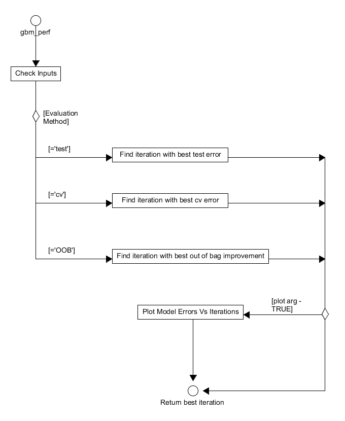 Figure 17. Activity diagram for the evaluation of the performance of a trained gbm model.
Using a previously fitted GBMFit object, the system provides an API through the gbmt_plot function to calculate and plot the marginal influences of the predictor variables on the fitted model.
When called the system will again check the user has provided the correct inputs. If the iteration at which the marginal influence is to be calculated exceeds the number in the original model fit then the requested iteration is set to the final iteration of the fit. The system only supports plotting of the marginal influences for up to 3 predictor variables, if more are examined then the return_grid parameter is set to TRUE and no plots will be displayed. After these checks, the grid of points at which the marginal influence of the selected predictors will be evaluated is constructed and the appropriate back-end function (in this case gbm_pred in gbmentry.cpp) is called. The output from this call is the marginal influence of each predictor that is then joined to the grid of evaluation points constructed earlier. If the return_grid parameter is set to TRUE then this new grid structure is returned to the user and the function terminates. If it is FALSE, then the categorical/factor predictor values (in the grid) are converted to appropriate numerics and the names of the predictor variables are set. The marginal influences are then plotted with the specific plot functionality determined on the form of the predictors, i. e. originally continuous or a factor, and number of predictors selected. The whole procedure undertaken by gbmt_plot is displayed in Figure 18.
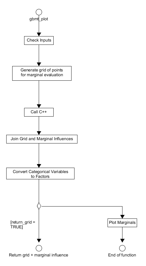 Figure 18. Activity diagram for the process of calculating the marginal effects of predictors - from the R layer perspective.
As alluded to in the previous Section, the system is structured around five main S3 classes that define the distribution, data, training parameters and variable properties associated with the model fit as well as the model fit itself. The first objects required for fitting a GBM model define the training parameters and the model distribution to be used in the fit. These public constructor methods for these objects are defined in training-params.r and gbm-dist.r respectively. During the fitting process, appropriate container classes for the data and variable properties are constructed and are ordered/validated using the training parameters and distribution objects, before all of these objects are wrapped up in a single GBMFit object at the end of the process. Beyond encapsulating the appropriate data, this design allows for much of the packages functionality to be implemented as S3 methods and where this is not necessary the inputs are now more homogenous and thus simpler to validate. These classes will be discussed individually with reference to the full system class diagram shown in Figure 19.
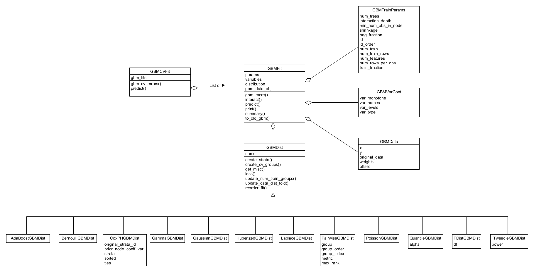 Figure 19. Full system class diagram for the R layer of the GBM package.
Much of the system's behaviour and functionality is dependent on the distribution selected by the user when training a gbm model. To reflect this the system contains a GBMDist class around which much of the systems functionality is built.
The GBMDist class itself is an abstract class that cannot be constructed directly within the system. Instead a call to gbm_dist constructor will create a specific distribution object that inherits from the GBMDist class, see Figure 20. This constructor is a wrapper constructor that firstly creates an empty distribution object of the appropriate derived class and then uses a S3 method, create-distributions.r, to construct the full distribution object which contains associated distribution specific data. This specific data is provided by the user through the call to gbm_dist and, along with this data, the constructed object will contain an appropriately populated name field .
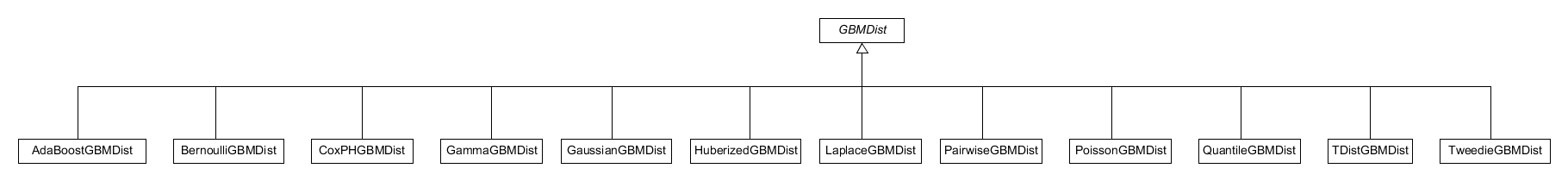 Figure 20. Class diagram of the S3 distribution classes used in the R layer.
The majority of functionality within the system is dependent on the distribution selected and this is reflected in the S3 nature of the system as well as switch statements on the objects name field that appear in simpler control flows.
Notable examples of this dependence include: the implementation of strata (only for "CoxPH") as well as the validation of the response and ordering of the data, furthermore the Bernoulli distribution offers stratification of responses during cross-validation. The distribution object also determines how groupings in data are handled, if it all (this is only relevant if "Pairwise" is selected), and the extraction of distribution specific data is also distribution specific (this is handled by the internal method get_misc()). Beyond this, lots of helper functions within the package are dependent on the constructed distribution object, examples include: determining the labels of various performance plots and the calculating the appropriate scaling of the fitted model predictions. The primary S3 methods associated with this class are shown along with the distribution dependent data in Figure 19.
Model parameters that define how the model will be trained are stored within the GBMTrainParams object which can be constructed by calling the training_params function (see training-params.r). This is a simple data object that is primarily used for storage of important GBM model fitting parameters such as: the number of boosted trees to fit, the maximum depth of each fitted tree, the number of training observations and the observation ids. The construction of the object takes a list of named parameter inputs and then simply stores them in a named argument list. During the construction process, the number of rows per observation along with the id order are determined and stored within the object. The GBMData has its predictors and response ordered according to the observation id order as part of the pre-processing in gbmt_fit. Post model-fitting, this object is stored as a field in GBMFit and is used to check inputs to other functions or control process flow as well as provide arguments for further calculation, methods such as gbm_more() illustrate the latter use.
The GBMData class is another simple object that is created by passing the covariate data, response data along with the response weights and offsets to the constructor defined in gbm-data.r. This constructor is a not accessible to the user and is instead called during the gbmt_fit pre-processing. Once created, the pre-processing in gbmt_fit converts categorical data stored within the object before ordering it ordered according to any groups present and the observation id. The order of the predictors is then determined and stored in the x_order field within the object. The GBMData object then plays a key role in the construction of the appropriate strata and the ordering of observations for CoxPH boosted models. If cross-validation is undertaken the data within the object is split and re-joined. The object is unpacked to supply appropriate arguments the call to the back-end. It is an object that can be stored, optionally, within the fitted model for access later so the user does not need to re-supply data but its role within the system is a primarily as a container during the fitting process.
This class is also a simple container class defined in variable-properties.r that stores data associated with the covariates used for fitting. This class cannot be constructed directly by the user and instead is produced through the model fitting process. It is initialized during the pre-processing of gbmt_fit where the variable names along with the monotonicity and GBMData object are used to initialize it. During contruction, the covariate variable type and number of levels (0 if continuous and a positive integer otherwise) associated with each variable are determined and stored in the object. The object is not used further in the process until its properties are unpacked as arguments to the back-end C++ call. After fitting, it is stored in the GBMFit object and is accessed by other functionality to extract predictor variable information, typical information required by other functions is the total number of variables used in the fit, see gbm-summary.r, or the type of variable each covariate is. This class has no S3 methods associated directly with it, this is shown in Figure 19.
The GBMFit class contains the output from the call to the gbm fitting functionality in C++ back-end, along with associated training parameters, variable containers and distribution classes used in the model fitting process. It also contains details of the user call, cross validation details (such as the number of folds used) and the parallelization parameters used in its construction. The output of a call to gbmt_fit this object is primarily used in further calculations by the user. The user may evaluate the models performance via gbm_perf as well as make predictions on new predictor data through its predict method. Additional boosted iterations may be added to the model through the gbm_more method and the marginal influences of the various predictors can be calculated by passing the object to gbmt_plot. Finally, it has an interact method that calculates the relevance of interactions between predictors in the fit as well as print and summary methods to display the model object. Outside of these cases, the object can be unpacked and its constituent data objects used in other functions within the system, i . e. the loss method is associated with the fit's GBMDist object and the model predictions.
When fitting a model it should be noted that gbmt and gbmt_fit provide an API for the parallelization of the underlying
tree boosting code. This parallelization is achieved using OpenMP and can be activated by passing a gbmParallel object, defined in gbm-parallel.r, to the par_details argument in gbmt and gbmt_fit. More specifically, this object stores data in appropriately named fields that set the number of thread to be used and the size of "chunks" to be used in array scans by the back-end during fitting. It should be noted that some experimentation as to the optimal configuration for a given set-up may be required.
To use the GBM package it is necessary to install a version of R on
your system, preferably 3.2 or higher. With R installed, the GBM
package may be installed by opening up a R terminal and using the
install.packages("gbm") command to install the package.
The system is subject to two types of testing: black-box system/acceptance tests
and unit testing. These tests are designed to run
with the testthat package and ship with the GBM package in /tests/
folder. The package can be checked using R CMD check <built package> which will automatically run all of the tests within it and
report any warnings or errors.
The package has a series of unit and black box system tests which
check that the package is operating as expected. The R layer of the
package has tests for nearly every piece of functionality. These tests check: the piece of
functionality's response to undesired inputs as well as its outputs
when correct inputs are provided. This ensures that all of the "work" and functionality provided by the
R layer, for every distribution available, is behaving as expected. On the other hand, the black box system tests check the overall behaviour of the package under using a variety of 'sanity test cases'. These tests primarily focus on the
Gaussian, Bernoulli and CoxPH distributions but additional tests, such as checking the effects
of the offset parameter, touch all distributions implemented in the
package. Using the covr package, the travis CI server automatically
collects code coverage data and sends it to coveralls.io. As of
11/08/2016 this coverage is at 91.57%, with high coverage levels for both the R
and C++ layers. This coverage statistic was taken directly from the Travis-CI build
and may not have transferred correctly to the badge on the repository's main page.
It should be noted that this coverage tool is not perfect and tends to underestimate the code
coverage. In particular, when working on the underlying C++ layer, it tends to miss header files
and inlined code which are exercised. The tests do miss some node functionality such as PrintSubTree and
GetVarRelativeInfluence and they do not touch many unhappy/error throwing paths
in the underlying C++. That being said, even without direct tests on the underlying C++,
most of the critical paths are exercised with the tests provided.
Finally, the C++ layer itself can now be tested using R's testthat
package thanks to a recent update. These unit tests have yet to be
written due to high coverage obtained through appropriate R API calls but they would provide
further re-assurance that each component in the C++ layer is behaving as expected.