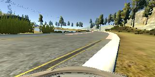
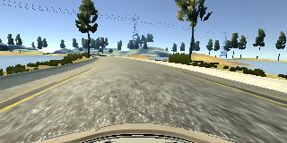
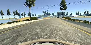
This repository contains starting files for the Behavioral Cloning Project.
In this project, I use deep neural networks and convolutional neural networks to clone driving behavior, train, validate and test a model using Keras. The model output's a steering angle to an autonomous vehicle.
This project uses a simulator provided by Udacity https://github.com/udacity/self-driving-car-sim where you can steer a car around a track for data collection. I used image data and steering angles to train a neural network and then use this model to drive the car autonomously around the track.
There are five key files:
- model.ipynb (script used to create and train the model)
- drive.pydrive.py (script to drive the car )
- model.h5(a trained Keras model)
- run10.mp4 (a video recording of the vehicle driving autonomously around the track for at least one full lap)
- README (this readme file has the write up for the project!)
The goals / steps of this project are the following:
- Use the simulator to collect data of good driving behavior
- Design, train and validate a model that predicts a steering angle from image data
- Use the model to drive the vehicle autonomously around the first track in the simulator. The vehicle should remain on the road for an entire loop around the track.
- Summarize the results with a written report
This lab requires:
The lab enviroment can be created with CarND Term1 Starter Kit. Click here for the details.
The following resources can be found in this github repository:
- drive.py
- video.py
- writeup_template.md
Usage of drive.py requires you have saved the trained model as an h5 file, i.e. model.h5. See the Keras documentation for how to create this file using the following command:
model.save(filepath)Once the model has been saved, it can be used with drive.py using this command:
python drive.py model.h5The above command will load the trained model and use the model to make predictions on individual images in real-time and send the predicted angle back to the server via a websocket connection.
Note: There is known local system's setting issue with replacing "," with "." when using drive.py. When this happens it can make predicted steering values clipped to max/min values. If this occurs, a known fix for this is to add "export LANG=en_US.utf8" to the bashrc file.
python drive.py model.h5 run1The fourth argument, run1, is the directory in which to save the images seen by the agent. If the directory already exists, it'll be overwritten.
ls run1

[2017-01-09 16:10:23 EST]  12KiB 2017_01_09_21_10_23_424.jpg
[2017-01-09 16:10:23 EST]  12KiB 2017_01_09_21_10_23_451.jpg
[2017-01-09 16:10:23 EST]  12KiB 2017_01_09_21_10_23_477.jpg
[2017-01-09 16:10:23 EST]  12KiB 2017_01_09_21_10_23_528.jpg
[2017-01-09 16:10:23 EST]  12KiB 2017_01_09_21_10_23_573.jpg
[2017-01-09 16:10:23 EST]  12KiB 2017_01_09_21_10_23_618.jpg
[2017-01-09 16:10:23 EST]  12KiB 2017_01_09_21_10_23_697.jpg
[2017-01-09 16:10:23 EST]  12KiB 2017_01_09_21_10_23_723.jpg
[2017-01-09 16:10:23 EST]  12KiB 2017_01_09_21_10_23_749.jpg
[2017-01-09 16:10:23 EST]  12KiB 2017_01_09_21_10_23_817.jpg
...
The image file name is a timestamp of when the image was seen. This information is used by video.py to create a chronological video of the agent driving.
python video.py run1Creates a video based on images found in the run1 directory. The name of the video will be the name of the directory followed by '.mp4', so, in this case the video will be run1.mp4.
Optionally, one can specify the FPS (frames per second) of the video:
python video.py run1 --fps 48Will run the video at 48 FPS. The default FPS is 60.
Here I will consider the rubric points individually and describe how I addressed each point in my implementation.
Node:
On my first iteration, I tried using a basic fully connected neural network as a default baseline starting point to get the data feed, pre-processing, training, output/ validation flows working.
2. Submission includes functional code Using the Udacity provided simulator and my drive.py file; the car can be driven autonomously around the track by executing
Python drive.py model.h5
The model.ipynb model.ipynb file contains the code for training and saving the convolution neural network. The file shows the pipeline I used for training and validating the model, and it contains comments to explain how the code works.
My initial approach was to use a fully connected neural network, but I quickly switched to a model used by Comma.ai at https://github.com/commaai/research/blob/master/train_steering_model.py, as my car was drifting off of the driving track.
The only change that i made to the model was I changed the Exponential Linear Activation to a Leaky ReLU activation. Leaky ReLUs allow a small, non-zero gradient when the unit is not active. If, for whatever reason, the output of a ReLU is consistently 0 (for example, if the ReLU has a large negative bias), then the gradient through it will consistently be 0. The error signal backpropagated from later layers gets multiplied by this 0, so no error signal ever passes to earlier layers. The ReLU has died. This small change seemed to improve the performance of the model (though this was mixed in with Data Augmentation from the Left & Right Cameras)
A model summary is as follows:
### INITIALIZE Keras sequential model
model = Sequential()
###Crop the images to remove extraneous information, focus on the immediate road ahead
model.add(Cropping2D(cropping=((70,25), (0,0)), input_shape=(160,320,3)))###Pre-process the data, center the data
### Normalize the model
model.add(Lambda(lambda x:x/127.5-1,input_shape=(160,320,3) ))

### USE THE MODEL DEFINED IN COMMA.AI Steering model
#https://github.com/commaai/research/blob/master/train_steering_model.py
model.add(Convolution2D(16, 8, 8, subsample=(4, 4), border_mode="same"))
model.add(LeakyReLU(alpha=.001))   # add an advanced activation
#model.add(ELU())
model.add(Convolution2D(32, 5, 5, subsample=(2, 2), border_mode="same"))
model.add(LeakyReLU(alpha=.001))   # add an advanced activation
#model.add(ELU())
model.add(Convolution2D(64, 5, 5, subsample=(2, 2), border_mode="same"))
model.add(Flatten())
model.add(Dropout(.2))
model.add(LeakyReLU(alpha=.001))   # add an advanced activation
#model.add(ELU())
model.add(Dense(512))
model.add(Dropout(.5))
model.add(LeakyReLU(alpha=.001))   # add an advanced activation
#model.add(ELU())
model.add(Dense(1))
### END COMMA.AI MODEL
### COMPILE USING ADAM OPTIMIZER, SO THAT LEARNING RATE DOESNT HAVE TO BE SET MANUALLY
model.compile(optimizer="adam", loss="mse")
I split my sample data into training and validation data. Using 80% as training and 20% as validation. train_samples, validation_samples = train_test_split(samples, test_size=0.2)
The model used an Adam optimizer, so the learning rate was not tuned manually.
I trained the vehicle by running it for 2 laps on the First course, and 1 lap over the 2nd course. This was not sufficient to keep the car within the boundaries of the course. The vehicle kept wandering off at 3 distinct points:
- When it found a white/ grey edge on the road.
- When it found a black edge on the road, on the bridge.
- When it approached brown/ sandy areas which were not clearly marked.
- When it happened to line up on a white edge.
NOTE: I cropped the training images before the normalization steps to save normalization operations on the part of the image that would anyways be cropped.
###Crop the images to remove extraneous information, focus on the immediate road ahead
model.add(Cropping2D(cropping=((70,25), (0,0)), input_shape=(160,320,3)))###Pre-process the data, center the data
The basic training on the laps was good enough to keep the vehicle within the track initially and then when it detected the red and white markings at sharp curves.
Initially, I started by using only the center camera images for training. With this, even though I was able to complete driving across the entire track, my vehicle drifted a few times on the edge of the tracks which is considered unsafe driving.
When I added in training to include the Left & Right Camera images, with a Steering correction factor of +0.2 for the left images and -0.2 for the right images, the vehicle was able to complete the track without wandering onto the edges. A correction factor was required because the left and right camera images are closer to the edges of the driving track.
TO fix the wandering problem in the 3 mentioned areas, I trained the vehicle by recording recovery manouvers by showing it to take sharp steering angles away from the white, grey and black edges. I also trained the vehicle to take sharp recovery angles when it landed on sandy/ brown patches. Finally, I trained the vehicle to start on the white boundaries and then recover inwards towards the tracks.
An example of training the vehicle to take sharp steering angles away from boundaries is show here [
In addition to these training strategies, I also augmented the data by flipping the images so it could learn behavior for both steering directions.
An example of the captured image and flipped image can be found here
In crossing the bridge, it helped to train the vehicle to stay away from the black edges by weaving an "S" curve across the bridge to train it to take medium steering angles to recover away from black edges.
A key part of the training strategy involved using the generator function in keras/ python. Once significant amount of images had been collected, my laptop was running out of memory to load all the images in memory [8GB Mac PRO]. Instead of switching to a more powerful machine on AWS or switching to a GPU instance, I used generators to load images as and when needed and available. This allowed me to complete the training process smoothly.
#setup generators, feed data in batches of 32 images to conserve memory
train_generator = generator(train_samples, batch_size=32)
validation_generator = generator(validation_samples, batch_size=32)
###SETUP GENERATOR FUNCTION TO STREAM DATA INSTEAD OF PRE-LOADING INTO MEMORY
def generator(samples, batch_size=128):
  ....
  yield sklearn.utils.shuffle(inputs, outputs)
I started with a generic dense network, which didnt work too well. I looked at the advanced Nvidia Architecture, but wanted to see if there was an easier fix, since I did not have access to the GPU. The Comma.AI steering model seemed like a good compromise between too simple and too complex of a network.
The vehicle made it just fine through multiple rounds of track 1 with this model, with the training strategy mentioned above.
A video of the vehicle driving along the track can be found here in the file run10.mp4.
I initially violated the rules of safe driving by crossing over the lane edges, even though I managed to complete the entire track. Turns out it was a simple matter of adding in the Left & Right camera images into the training process to ensure the vehicle stuck to center of the lane driving.
Running model.summary() provided the following details of the Neural Network:
____________________________________________________________________________________________________
Layer (type)                     Output Shape          Param #     Connected to
====================================================================================================
cropping2d_1 (Cropping2D)        (None, 65, 320, 3)    0           cropping2d_input_1[0][0]
____________________________________________________________________________________________________
lambda_1 (Lambda)                (None, 65, 320, 3)    0           cropping2d_1[0][0]
____________________________________________________________________________________________________
convolution2d_1 (Convolution2D)  (None, 17, 80, 16)    3088        lambda_1[0][0]
____________________________________________________________________________________________________
leakyrelu_1 (LeakyReLU)          (None, 17, 80, 16)    0           convolution2d_1[0][0]
____________________________________________________________________________________________________
convolution2d_2 (Convolution2D)  (None, 9, 40, 32)     12832       leakyrelu_1[0][0]
____________________________________________________________________________________________________
leakyrelu_2 (LeakyReLU)          (None, 9, 40, 32)     0           convolution2d_2[0][0]
____________________________________________________________________________________________________
convolution2d_3 (Convolution2D)  (None, 5, 20, 64)     51264       leakyrelu_2[0][0]
____________________________________________________________________________________________________
flatten_1 (Flatten)              (None, 6400)          0           convolution2d_3[0][0]
____________________________________________________________________________________________________
dropout_1 (Dropout)              (None, 6400)          0           flatten_1[0][0]
____________________________________________________________________________________________________
leakyrelu_3 (LeakyReLU)          (None, 6400)          0           dropout_1[0][0]
____________________________________________________________________________________________________
dense_1 (Dense)                  (None, 512)           3277312     leakyrelu_3[0][0]
____________________________________________________________________________________________________
dropout_2 (Dropout)              (None, 512)           0           dense_1[0][0]
____________________________________________________________________________________________________
leakyrelu_4 (LeakyReLU)          (None, 512)           0           dropout_2[0][0]
____________________________________________________________________________________________________
dense_2 (Dense)                  (None, 1)             513         leakyrelu_4[0][0]
====================================================================================================
Total params: 3,345,009
Trainable params: 3,345,009
Non-trainable params: 0
To visualize the model, couple of additional package are required. On my mac, I first installed:
brew install graphviz
pip install graphviz
conda install -c anaconda pydot
Then I generated the visualization of the model:
from keras.utils.visualize_util import plot
plot(model, to_file='model.png')


