summary | contents | usage | running the notebooks | citation | issues | license


This repository contains the notebooks used to generate the examples shown in Chapter 2 of the thesis "Electromagnetic methods for imaging subsurface injections" by Lindsey J. Heagy.
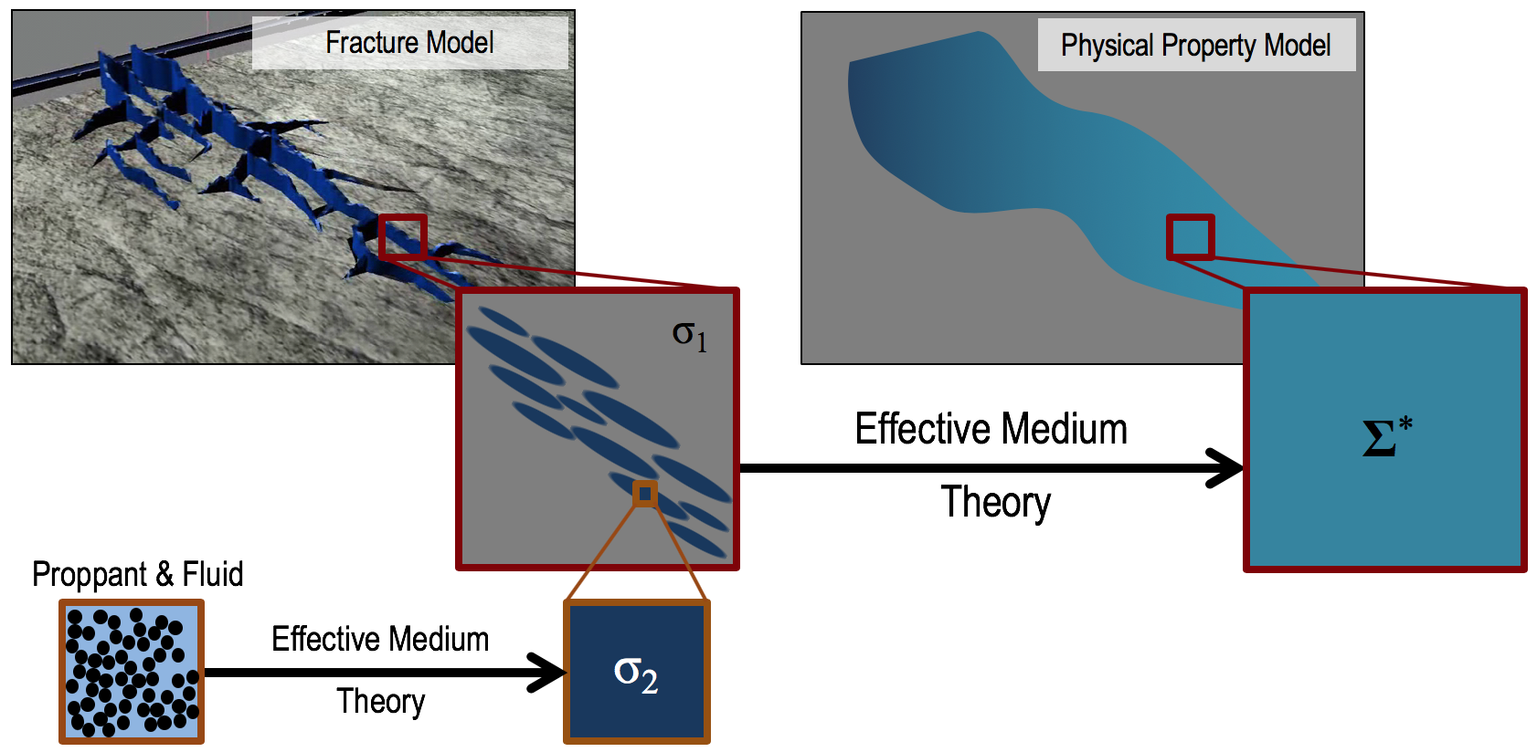
In hydraulic a fracturing operation, fluid is injected into the reservoir to fracture the rock and provide pathways for hydrocarbons to flow. In order to keep the fracture pathways open, sand or ceramic particles, known as proppant are also injected. One of the unknowns in fracturing operations is where the proppant goes. If the proppant were electrically conductive (e.g. by coating it with graphite), then electromagnetic (EM) methods can be used to detect the proppant. The first step to examining the feasibility of using EM methods for delineating the propped region of the reservoir is construcing an electrical conductivity model that can be used for numerical simulations.
To estimate the conductivity of afractured volume of rock, I use effective medium theory in two steps. First, I estimate the conductivity of a mixture of proppant and fluid and second, I estimate the conductivity of a fractured volume of rock. In the final notebook, I perform a simulation of cross-well electromagntic data to demonstrate feasibility of using electromagnetic methods for detecting a propped, fractured volume of rock.
The notebooks can be run online through mybinder or azure notebooks.
To run them locally, you will need to have python installed, preferably through anaconda.
You can then clone this reposiroty. From a command line, run
git clone https://github.com/simpeg-research/heagy-2018-fracture-physprops.git
Then cd into the heagy-2018-fracture-physprops
cd heagy-2018-fracture-physprops
To setup your software environment, we recommend you use the provided conda environment
conda env create -f environment.yml
source activate fracture-physprops-environment
alternatively, you can install dependencies through pypi
pip install -r requirements.txt
You can then launch Jupyter
jupyter notebook
Jupyter will then launch in your web-browser.
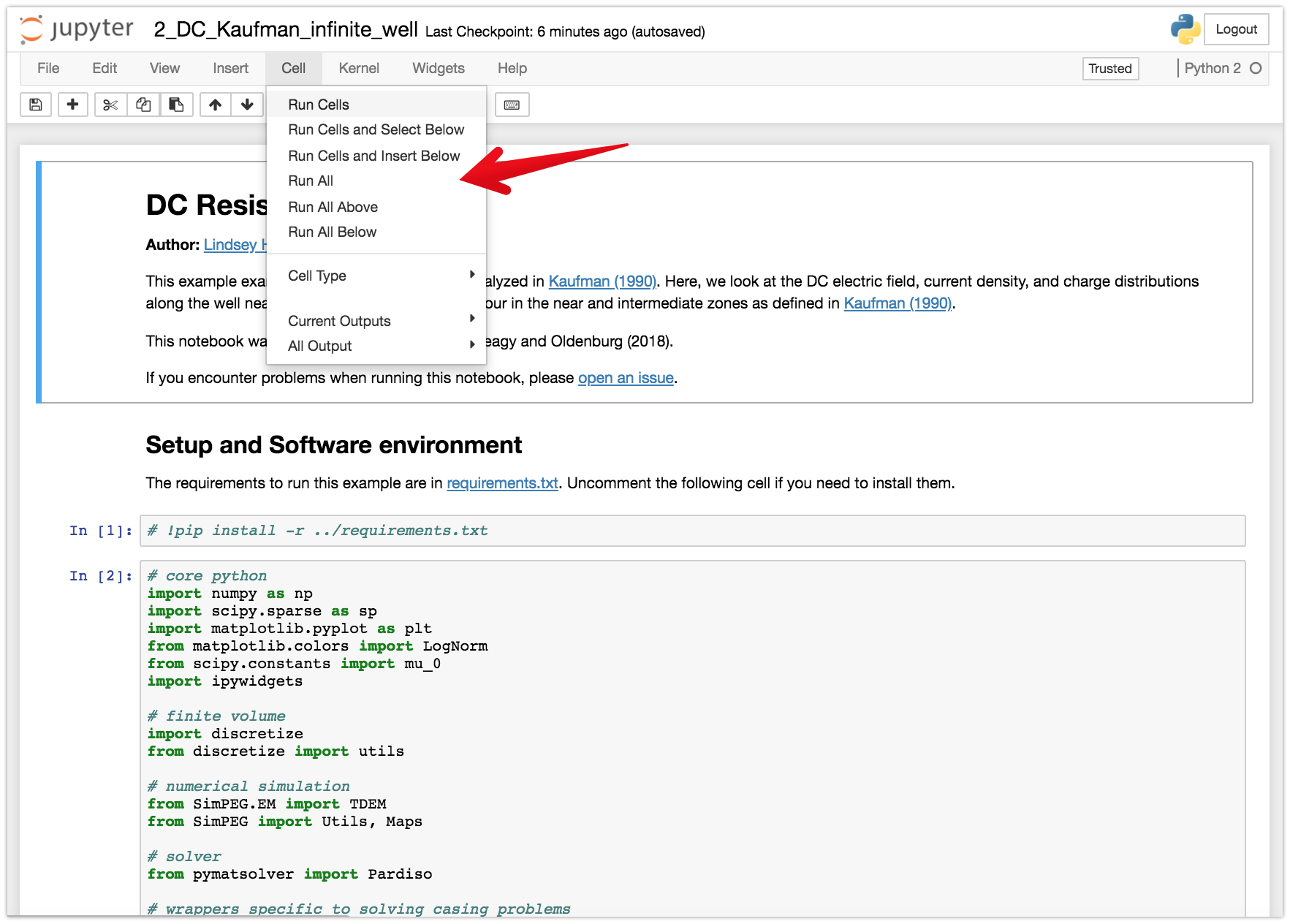
Each cell of code can be run with shift + enter or you can run the entire notebook by selecting cell, Run All in the toolbar.
For more information on running Jupyter notebooks, see the Jupyter Documentation
coming soon...
If you run into problems or bugs, please let us know by creating an issue in this repository.
These notebooks are licensed under the MIT License which allows academic and commercial re-use and adaptation of this work.