-
Notifications
You must be signed in to change notification settings - Fork 54
Example: Bayer Filter Demosaic
To see the whole code of this example: link
The Bayer filter is a common approach for designing a colour filter array for a camera.
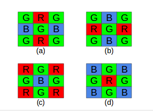
In the Bayer filter array, the camera is designed to have 1 sensor to capture Red colours, 2 sensors to capture Green colours and 1 sensor to capture Blue colour. Half of the sensors are green since the human eyes is more sensible to green colours. There are 4 different patterns how the filter array can be designed RGGB, BGGR, GBGR, GRGB. In the image below [1], it is possible to see how a Bayer filter array is usually designed.
![Bayer Filter] (https://raw.githubusercontent.com/wiki/codeplaysoftware/visioncpp/images/bayer_image.png)
This tutorial aims to show implement details of the demosaic method in VisionCpp framework. The demosaic method converts the Bayer filter array to RGB. This method computes an interpolation for the 2 missing channels in each pixel. Since it is done per pixel, it fits well for the parallel implementation. Only one kernel is needed. As mentioned before, there are four different patterns of the Bayer filter. For this example we are going to use the RGGB pattern.
The code below shows the header of our demosaic functor:
struct BayerRGGBToBGR {
  template <typename T>
  visioncpp::pixel::U8C3 operator()(T bayer) {
    ...
  }
};There are 4 different cases that can be used for R and B channels creation.

Since we know in advance the pattern we are using (RGGB), we can know the current case by the index.
- All G1 values will be at even rows and odd columns (Case (a)).
- All G2 values will be at odd rows and even columns (Case (b)).
- All B values will be at odd rows and odd columns (Case (c)).
- All R values will be at even rows and even columns (Case d).
// finding the pattern based on the index
int _case = 0;
if (bayer.I_r % 2 == 0 && bayer.I_c % 2 == 0) {
  _case = 1; // Case (d)
} else if (bayer.I_r % 2 == 0 && bayer.I_c % 2 == 1) {
  _case = 2; // Case (b)
} else if (bayer.I_r % 2 == 1 && bayer.I_c % 2 == 0) {
  _case = 3; // Case (a)
} else {
  _case = 4;  // Case (b)
}
In the Figures (a) and (b) we simply get the average of the two nearest values. In the Figure (c) to compute the R channel, we need to get the average of the 4 Red neighbours. Similar done for B in the Figure (d).
Let's see in the code how it is done.
- Case (a)
// Getting the R values
uchar R1 = bayer.at(bayer.I_c, bayer.I_r - 1)[0];
uchar R2 = bayer.at(bayer.I_c, bayer.I_r + 1)[0];

// Getting the B values
uchar B1 = bayer.at(bayer.I_c - 1, bayer.I_r)[0];
uchar B2 = bayer.at(bayer.I_c + 1, bayer.I_r)[0];

// R
uchar R = (R1 + R2) / 2;

// B
uchar B = (B1 + B2) / 2;- Case (b)
// Getting the R values
uchar R1 = bayer.at(bayer.I_c - 1, bayer.I_r)[0];
uchar R2 = bayer.at(bayer.I_c + 1, bayer.I_r)[0];

// Getting the B values
uchar B1 = bayer.at(bayer.I_c, bayer.I_r - 1)[0];
uchar B2 = bayer.at(bayer.I_c, bayer.I_r + 1)[0];

// R
uchar R = (R1 + R2) / 2;

// B
uchar B = (B1 + B2) / 2;- Case (c)
// Getting the R values
uchar R1 = bayer.at(bayer.I_c - 1, bayer.I_r - 1)[0];
uchar R2 = bayer.at(bayer.I_c + 1, bayer.I_r - 1)[0];
uchar R3 = bayer.at(bayer.I_c + 1, bayer.I_r + 1)[0];
uchar R4 = bayer.at(bayer.I_c - 1, bayer.I_r + 1)[0];

// R
uchar R = (R1 + R2 + R3 + R4) / 4;

// B (center pixel)
uchar B = bayer.at(bayer.I_c, bayer.I_r)[0];- Case (d)
// Getting the B values
uchar B1 = bayer.at(bayer.I_c - 1, bayer.I_r - 1)[0];
uchar B2 = bayer.at(bayer.I_c + 1, bayer.I_r - 1)[0];
uchar B3 = bayer.at(bayer.I_c + 1, bayer.I_r + 1)[0];
uchar B4 = bayer.at(bayer.I_c - 1, bayer.I_r + 1)[0];

// B
uchar B = (B1 + B2 + B3 + B4) / 4;

// R (center pixel)
uchar R = bayer.at(bayer.I_c, bayer.I_r)[0];
VisionCpp is Column-major, so the first parameter of the matrix access the column, and the second access the row.
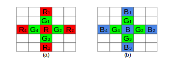
To implement the G channel interpolation, we have two patterns:

-
Case (a) : For the case in the Figure (a) we have the following interpolation formula

-
Implementing the above equation in VisionCpp:
    // Init G
    uchar G;

    // Getting G values
    uchar G1 = bayer.at(bayer.I_c, bayer.I_r - 1)[0];
    uchar G2 = bayer.at(bayer.I_c + 1, bayer.I_r)[0];
    uchar G3 = bayer.at(bayer.I_c, bayer.I_r + 1)[0];
    uchar G4 = bayer.at(bayer.I_c - 1, bayer.I_r)[0];

    // Getting R values
    uchar R1 = bayer.at(bayer.I_c, bayer.I_r - 2)[0];
    uchar R2 = bayer.at(bayer.I_c + 2, bayer.I_r)[0];
    uchar R3 = bayer.at(bayer.I_c, bayer.I_r + 2)[0];
    uchar R4 = bayer.at(bayer.I_c - 2, bayer.I_r)[0];

    // G
    if (abs(R1 - R3) < abs(R2 - R4)) {
       G = (G1 + G3) / 2;
    } else if (abs(R1 - R3) > abs(R2 - R4)) {
       G = (G2 + G4) / 2;
    } else {
       G = (G1 + G2 + G3 + G4) / 4;
}-
Case (b) : For the case in the Figure (b) we have the following interpolation formula

-
Implementing the above equation in VisionCpp:
    // Init G
    uchar G;

    // Getting G values
    uchar G1 = bayer.at(bayer.I_c, bayer.I_r - 1)[0];
    uchar G2 = bayer.at(bayer.I_c + 1, bayer.I_r)[0];
    uchar G3 = bayer.at(bayer.I_c, bayer.I_r + 1)[0];
    uchar G4 = bayer.at(bayer.I_c - 1, bayer.I_r)[0];

    // Getting B values
    uchar B1 = bayer.at(bayer.I_c, bayer.I_r - 2)[0];
    uchar B2 = bayer.at(bayer.I_c + 2, bayer.I_r)[0];
    uchar B3 = bayer.at(bayer.I_c, bayer.I_r + 2)[0];
    uchar B4 = bayer.at(bayer.I_c - 2, bayer.I_r)[0];

    // Assign G
    if (abs(B1 - B3) < abs(B2 - B4)) {
       G = (G1 + G3) / 2;
    } else if (abs(R1 - B3) > abs(B2 - B4)) {
       G = (G2 + G4) / 2;
    } else {
       G = (G1 + G2 + G3 + G4) / 4;
}- Since we created the Bayer filter functor ( node ), we can use it in the expression tree as follows:
  // Init input node with the bayer image
    auto in_node =
        visioncpp::terminal<visioncpp::pixel::U8C1, COLS, ROWS,
                            visioncpp::memory_type::Buffer2D>(bayer.data);

    // Init output node
    auto out_node =
        visioncpp::terminal<visioncpp::pixel::U8C3, COLS, ROWS,
                            visioncpp::memory_type::Buffer2D>(output_ptr.get());

    // apply demosaic method (Bayer RGGB to BGR)
    auto bgr =
        visioncpp::neighbour_operation<BayerRGGBToBGR, 2, 2, 2, 2>(in_node);

    // assign to the host memory
    auto k = visioncpp::assign(out_node, bgr);

    // execute
    visioncpp::execute<visioncpp::policy::Fuse, 32, 32, 16, 16>(k, dev);
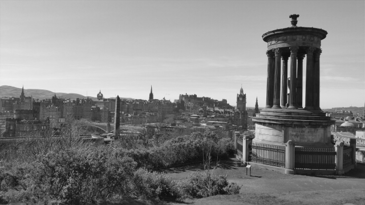
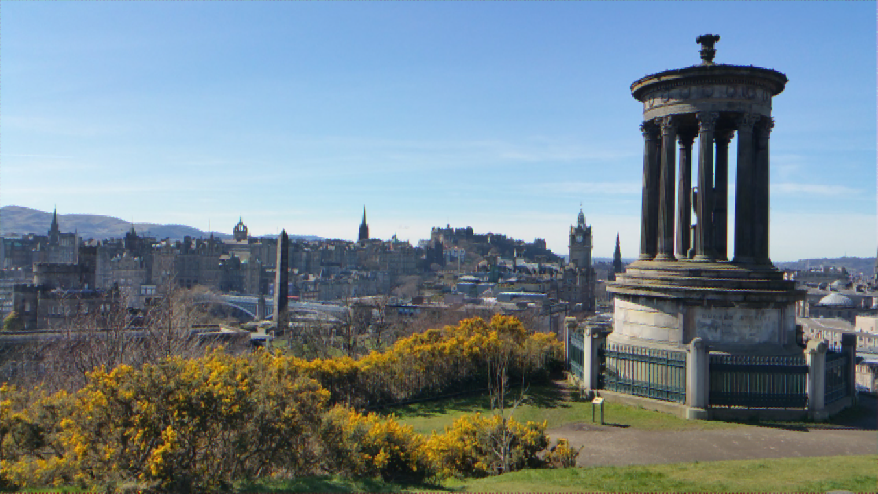
The image below show the raw Bayer format image ( left ) and the result image ( right ) after the demosaic node was applied.
| Reference Image [2] | Demosaic Image |
|---|---|
 |
 |
[1] https://en.wikipedia.org/wiki/Bayer_filter#/media/File:Bayer_pattern_on_sensor.svg