Fluid Simulator

Overview

Fluid Simulator implements a physics simulator that visualizes the behavior of fluids in an interactive environment. The algorithm is based on the Navier-Stokes equations which define the fluid flow in physics. Some other mathematical methods such as Gauss-Seidel relaxation, Hodge decomposition and Poisson's equation were also employed in the algorithm.

Feel free to browse at Fluid Simulator.

Features & Implementation

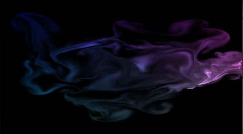
The simulator allows user to customize their own fluid field by being able to manipulate the viscosity, diffusion rate and added density. One can also change the resolution and number of iterations for Gauss-Seidel method for sharper, more accurate simulations.

Note: High resolution and iterations might be computationally heavy and slow depending on the computer used!

Density and Velocity Steps

2 main fields that represent the state of the fluid are density field and velocity field. Velocity field is represented by 2 different arrays(speed in x direction and y direction) as velocity is a vectoral quantity. At each time step density and velocity fields are recalculated according to the approximation of the Navier-Stokes equations.

Node: The scalar quantities for the mentioned fields will be referred to as:

• Density => d
• Speed in x direction => u
• Speed in y direction => v

Gauss-Seidel Solver

As mentioned earlier the Gauss-Seidel relaxation is used in solving Poisson's equation and Navier-Stokes equations. Three main methods used in calculation of the velocity and density fields are diffuse, advect and project.

Diffusion

The method diffuse which calculates the diffusion of the scalar quantities d, u, v. The method uses Gauss-Seidel relaxation which is implemented as follows:

function gaussSeidel(b, x, x0, diff){
  let a = dt * diff;

  for(let k = 0; k < iter; k++){
    for(let i = 1; i <= N; i++){
      for(let j = 1; j <= N; j++){
        let neighborSum = x[IX(i-1, j)] + x[IX(i+1, j)] + x[IX(i, j-1)] + x[IX(i, j+1)];
        x[IX(i, j)] = (x0[IX(i, j)] + a * neighborSum) / (1 + 4 * a);
      }
    }
    setBoundary(b, x);
  }
}

Advection

Advection is the transfer of velocities and densities across the field. A model of advection is used to create the flow of the fluid as it's velocity and density changes. The velocity and time step are used to determine the next cell each particle is going to be in at next time slice. After determining the correct cell for each particle, the fields d, u, v are modified accordingly.

Projection

Projection on velocity field(as it is a vectoral field) is necessary for conservation of the mass. Projection is used to calculate the directional changes in velocity field while conserving the mass of the system. Using Hodge decompositions result: every velocity field is the sum of a mass conserving field and a gradient field, we subtract velocity field from the gradient to find the mass conserving field. We can use Poisson's equation to calculate the mass conserving field.

Here's the project method:

function project(u, v, p, div){
    for(let j = 1; j <= N; j++){
        for(let i = 1; i <= N; i++){
          let neighborSum = u[IX(i+1, j)] - u[IX(i-1, j)] + v[IX(i, j+1)] - v[IX(i, j-1)];
          div[IX(i, j)] = -0.5 * neighborSum / N;

          p[IX(i, j)] = 0;
        }
    }
    setBoundary(0, div);
    setBoundary(0, p);

    for(let k = 0; k < iter; k++){
      for(let i = 1; i <= N; i++){
        for(let j = 1; j <= N; j++){
          let neighborSum = p[IX(i-1, j)] + p[IX(i+1, j)] + p[IX(i, j-1)] + p[IX(i, j+1)];
          p[IX(i, j)] = (div[IX(i, j)] + neighborSum) / 4;
        }
      }
      setBoundary(0, p);
    }
    setBoundary(0, p);

    for(let j = 1; j <= N; j++){
        for(let i = 1; i <= N; i++){
            u[IX(i, j)] -= 0.5 * N * (p[IX(i+1, j)] - p[IX(i-1, j)]);
            v[IX(i, j)] -= 0.5 * N * (p[IX(i, j+1)] - p[IX(i, j-1)]);
        }
    }
    setBoundary(1, u);
    setBoundary(2, v);
}

Potential Extensions

Enhance the API

The simulator's API can be improved for easier usage and integrations to other projects such as a fluid dynamics music visualizer etc.

Add Keyboard interactions

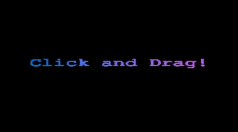
Currently the renderer is set to interaction with mouse click and drag. Another renderer that allows interaction through keyboard can be implemented.

Ability to determine custom color palette

A control to allow user to be able to change the color palette of the fluid renderer would allow more customization.