=====================
Simple ABC Tutorial will introduce you to inference via Approximate Bayesian Computation using the simple example of estimating the mean of a binomial distribution. You can choose to run the tutorial as is with the test case supplied herein, using 1 command line input. Alternatively, you can modify the analysis by editing 'input.csv' and run the tutorial multiple times in order to familiarize yourself with how different components influence the analysis.
Bayesian inference methods estimate unknown parameters while incorporating statistical uncertainty. Employing Bayesian inferences involves: (1) assuming a model and setting a prior probability distribution for the parameter of interest, (2) updating the prior distribution based on observed data in order to generate a posterior probability distribution for the parameter of interest. Updating the prior distribution requires the evaluation of a likelihood function, which is often computationally challenging. The evaluation of the likelihood function can become computationally intractable when the underlying model is complex. Motivation to consider more complex demographic models of natural populations has led to the development of methods that reduce the computational intensity of Bayesian inference by simplifying, or altogether circumventing evaluating the likelihood function (Marjoram & Tavare 2006).
Approximate Bayesian Computation (ABC) is one method that reduces the computational intensity of Bayesian inference by conducting simulations and calculating summary statistics, altogether avoiding the evaluation of a likelihood function. Generally, (1) a parameter value is sampled from the prior distribution, (2) a dataset is simulated under the assumed model, (3) summary statistics are calculated for the simulated dataset, (4) summary statistics calculated from the simulated and observed data are compared and if the simulated summary statistics are close enough to that of the observed that simulation is accepted, and (5) the posterior distribution for the parameter of interest is summarized from the accepted simulations and the parameter of interest and its credibility interval is estimated. There are 3 main methods for comparing the simulated and observed summary statistics, the model fitting step of the analysis (Beaumont 2010). The first method builds on a basic rejection algorithm, rejecting the simulated statistic if it falls outside a set tolerance threshold (Pritchard et al. 1999; Tavare et al. 1997).
Download or clone this (SimpleABCTutorial repository)! Requires:
Before experimenting with changing parameters in input.csv, follow the steps under implementation to confirm the tutorial is functional.
1. Populate the fields of 'input.csv'
- p: Parameter of true binomial distribution defining the probability of success. Takes floating points between 0.0 and 1.0.
- N: Parameter of true binomial distribution defining the number of trials. Takes integers, theoretically, without bound. However, keep in mind that at large values the binomial can be approximated by the normal distribution.
- sample_size: The number of random samples our observed and simulated datasets will contain. Takes integers. I encourage you to experiment, but start small (~20-50).
- posterior_size: The number of accepted parameter estimates we will accept before ending our analysis. Takes integers. Again, I encourage you to experiment, but start small (~100).
- method: Model fitting algorithm that will be used. At present a modified rejection algorithm indicated by rej is the only supported option
- sumstat: Summary statistic that will be used to summarize datasets for model fitting. Takes mean | median | mode.
2. At the command line, cd into the SimpleABCTutorial directory.
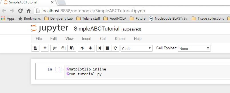
3. Enter the command: ipython notebook SimpleABCTutorial.ipynb
- A web browser will open with an active ipython notebook with 2 lines of code.
4. Immediately click the File tab in the left top corner and select the option to make a copy.
- Save the copy as with a new file name!
- Close the web tab of the original ipython notebook without any changes.
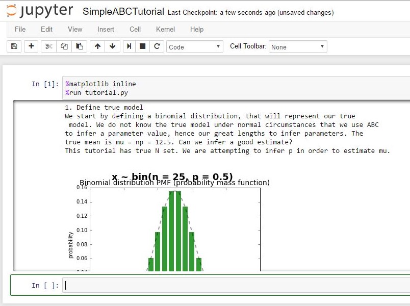
5. Hover your mouse pointer over the Cell tab of the ipython notebook and select Run.
- Your tutorial will appear below.
Simple ABC Tutorial 1.0 is written in Python3.5 as distributed in Anaconda. No dependencies outside of this distribution are required.
What to expect in future versions!
- implementation of another model fitting option, local linear regression adjustment of simulated summary statistics
- implementation model selection to compare parameter inference under models of binomial and normal distributions
Marjoram P, Tavare S (2006) Modern computational approaches for analysing molecular genetic variation data. Nature Reviews Genetics 7, 759-770.
Pritchard JK, Seielstad MT, Perez-Lezaun A, Feldman MW (1999) Population growth of human Y chromosomes: A study of Y chromosome microsatellites. Molecular Biology and Evolution 16, 1791-1798.
Tavare S, Balding DJ, Griffiths RC, Donnelly P (1997) Inferring coalescence times from DNA sequence data. Genetics 145, 505-518.
Math-y
Beaumont MA (2010) Approximate Bayesian Computation in Evolution and Ecology. In: Annual Review of Ecology, Evolution, and Systematics, Vol 41 (eds. Futuyma DJ, Shafer HB, Simberloff D), pp. 379-406.
Light
Csillery K, Blum MGB, Gaggiotti OE, Francois O (2010) Approximate Bayesian Computation (ABC) in practice. Trends in Ecology & Evolution 25, 410-418.