Steady state heat/temperature solver in 2d

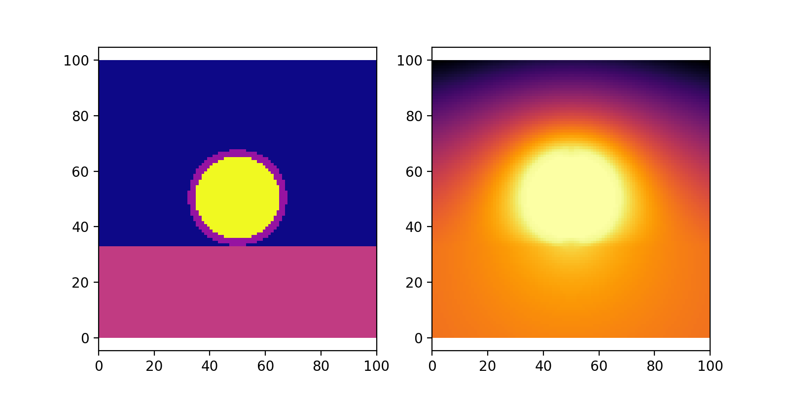
A specialized solver designed to find the steady-state temperature distribution in (2d rectangle) cross sections of walls with capillary heat exchangers. Capillary heat exchangers enable efficient use of heat pumps, if properly set up these systems require lower heating temperatures to achieve the required heat fluxes.

The solver utilizes a linear system of equations to model the temperature distribution within the wall cross section. It takes into account the geometry of the wall, including the presence of capillary heat exchangers and water regions, as well as boundary conditions such as heat flux, constant temperature or convective heat transfer.

The main function, fit_water_t, initializes the system and fits the required water temperature to achieve a target temperature and heat flux specified by the user. It iteratively solves the linear system using the scipy.spsolve function and adjusts the water temperature until convergence is achieved or the maximum number of iterations is reached. The resulting temperature distribution and the adjusted water temperature are returned. Additional functions, such as init_Ab and init_l, handle the initialization of the geometry matrix, coefficient matrix (A), and right-hand side vector (b) for the linear system.

Method

i use FDM to aproximate $\nabla (\lambda \nabla T ) = 0 $ and build a system of linear equations to solve for the stationary state.

The equation as solved:

with T as temperature(kelvion or celsisus)(i=y,j=x), k as thermal conductivity of the nodes own grid cell or neighbour with: T - top, B - bottom, L - left, R - right. Each of the terms describes a heat flux to a neighboring node.

Implemented boundary conditions and "ghost cells"

Bottom

Neumann Boundary Condition (Type II), requiers a ghost cell to impose the heat flux, this is where the padding comes in.

$\frac{\delta T}{\delta y}_{y=0} = \frac{q}{\lambda}$

Top

At the top boundary, a fixed temperature or convective boundary condition can be specified, simulating different scenarios encountered in practical applications. Fixed temperature dosent require an aditonal layer, just that the boundary layer is set to the fixed temperature. But convective boundary requires a ghost cell for the temperature at infinity and to impose the prescribed flux. The convection is described by:

$\frac{\delta T}{\delta y}_{y=top} = \alpha(T-T_0)$

With $\alpha$ as the convective constant, T as temperature of a boundary element of the medium and $T_0$ as temperature at infinity.

Sparse Arrays

Because the size of the coefficent matrix scalles as '(nxny, nxny)', it quiet quickly becomes too large as a numpy array to be held in ram.

for example np.zeros((100*1500,100*1500)) yields:

MemoryError: Unable to allocate 168. GiB for an array with shape (150000, 150000) and data type float64

But its mostly zeros - a sparse matrix, so scipy.sparse is used.

Examples in the notebook