| title | separator | verticalSeparator | theme | paginate |
|---|---|---|---|---|
Annotated S4 |
--- |
<!--v--> |
default |
true |
Sasha Rush (@srush_nlp) with Sidd Karamcheti
https://github.com/srush/annotated-s4
Based on research by Albert Gu, Karan Goel, and Christopher Ré.
-
Professor at Cornell / Researcher at Hugging Face
-
Open source projects
Caveat: Not a research talk, there will be bugs 🧑🔬
-
- Learn about a new ML architecture.
- Understand how JAX supports it.
-
- Debugging is still hard
- No NN standard
- Hard to reason about (for me)
-
- Seperate math from NN (facilitates testing)
- JIT is really impressive
- Lifted transformations are magic
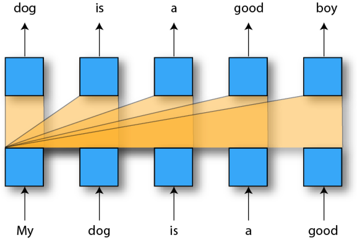
Birds-Eye: Learning over a list of elements (discrete or sampled signal)
-
Classification
Is the dog a good boy?
- Yes
-
Generation
The dog is a good _____
- Scales
$O(L^2)$ with length$L$ .
- Scales
$O(L)$ with length$L$ .
- A benchmark of extremely long sequence tasks (up to 16k tokens)
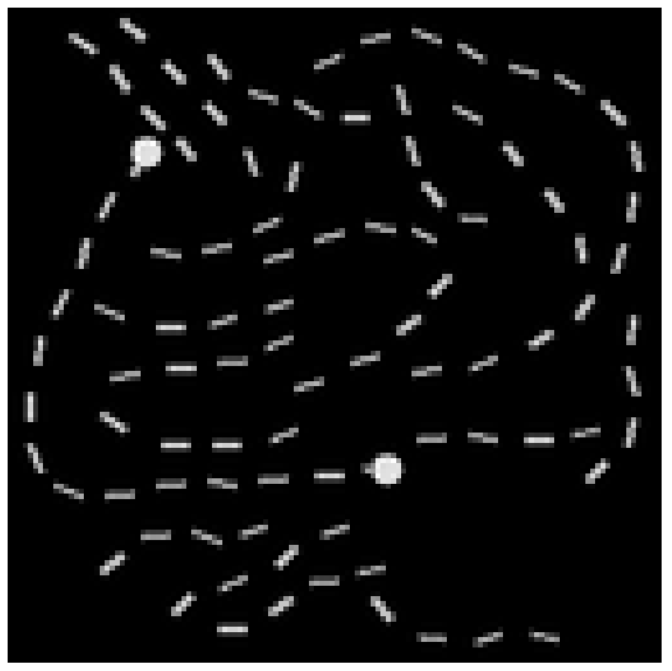
- Classification problem on linearized (one pixel at a time) image sequence.
Albert Gu, Karan Goel, and Christopher Ré.
- The model is quite mathematically complicated (want to test)
- Core operations required external libraries in Torch
- Follow-up work uses similar structure
- A concise pedagogical JAX / Flax implementation.
- A state space model maps a 1-D input signal
$u(t)$ to an$N$ -D latent state$x(t)$ before projecting to a 1-D output signal$y(t)$ .
-
$\boldsymbol{A}$ ,$\boldsymbol{B}$ ,$\boldsymbol{C}$ are parameters;$u$ input,$y$ output,$x$ state
def random_SSM(rng, N):
    a_r, b_r, c_r = jax.random.split(rng, 3)
    A = jax.random.uniform(a_r, (N, N))
    B = jax.random.uniform(b_r, (N, 1))
    C = jax.random.uniform(c_r, (1, N))
return A, B, C-
To discretize input sequence
$(u_0, u_1, \dots, u_{L-1})$ need a step size$\Delta$ representing$u_k = u(k \Delta)$ . -
One choice for discretization is a bilinear transform.
def discretize(A, B, C, step):
    I = np.eye(A.shape[0])
    BL = inv(I - (step / 2.0) * A)
    Ab = BL @ (I + (step / 2.0) * A)
    Bb = (BL * step) @ B
return Ab, Bb, C- Once discretized with step
$\Delta$ , the SSM can be viewed as a linear RNN,
def scan_SSM(Ab, Bb, Cb, u, x0):
    def step(x_k_1, u_k):
        x_k = Ab @ x_k_1 + Bb @ u_k
        y_k = Cb @ x_k
        return x_k, y_k

return jax.lax.scan(step, x0, u)-
Example from mechanics, mass on a spring
- forward position
$y(t)$ - force
$u(t)$ is applied to this mass - parameterized by mass (
$m$ ), spring constant ($k$ ), friction constant ($b$ )
- forward position
def example_mass(k, b, m):
    A = np.array([[0, 1], [-k / m, -b / m]])
    B = np.array([[0], [1.0 / m]])
    C = np.array([[1.0, 0]])
return A, B, C@partial(np.vectorize, signature="()->()")
def example_force(t):
x = np.sin(10 * t)
return x * (x > 0.5)def example_ssm(L=100):
ssm = example_mass(k=40, b=5, m=1)
# L samples of u(t).
step = 1.0 / L
ks = np.arange(L)
u = example_force(ks * step)
y = scan_SSM(*ssm, u)- Our Goal: Train a neural network with SSMs
- SSM RNNs: Fast for generation, but slow for training
- SSM CNNs: Slow for generation, but fast for training
- Initilization
- "Unroll" the RNN representation
- Form a
$L$ -length kernel
def K_conv(Ab, Bb, Cb, L):
    return np.array(
        [(Cb @ matrix_power(Ab, l) @ Bb).reshape() for l in range(L)]
)- Apply as a (non-cicular) convolution
def non_circular_convolution(u, K, nofft=False):
    if nofft:
        return convolve(u, K, mode="full")[: u.shape[0]]
    else:
        ud = np.fft.rfft(np.pad(u, (0, K.shape[0])))
        Kd = np.fft.rfft(np.pad(K, (0, u.shape[0])))
return np.fft.irfft(ud * Kd)[: u.shape[0]]-
$O(L \log L)$ training through FFT
Initialization with HiPPO
- Fast training, but random init does terribly. MNIST classification benchmark
$50%$ . - HiPPO initialization of
$\mathbf{A}$ improves this number to$98%$
def make_HiPPO(N):
    def v(n, k):
        if n > k:
            return np.sqrt(2 * n + 1) * np.sqrt(2 * k + 1)
        elif n == k:
            return n + 1
        else:
            return 0
    mat = [[v(n, k) for k in range(1, N + 1)] for n in range(1, N + 1)]
return -np.array(mat)- Recall
$x_k$ is an$N$ -dimensional hidden representation of an$L$ -step signal - HiPPO approximates state as
$N$ Legendre coefficients representing$u$ .
def example_legendre(N=8):
    u = (np.random.rand(N) - 0.5) * 2
    t = np.linspace(-1, 1, 100)
x = numpy.polynomial.legendre.Legendre(u)(t)- Everything is a modular testable function
- So far - no parameter, batches, NN nonsense
- In fact, mostly scalar modeling.
- SSM layer with Flax (still scalar!)
class SSMLayer(nn.Module):
    A: np.DeviceArray  # HiPPO
    N, L: int

    def setup(self):
        self.B = self.param("B", lecun_normal(), (self.N, 1))
        self.C = self.param("C", lecun_normal(), (1, self.N))
        self.step = np.exp(self.param("log_step", log_step_initializer(), (1,)))

        # Conv created each time during training
        self.ssm = discretize(self.A, self.B, self.C, step=self.step)
        self.K = K_conv(*self.ssm, self.L)

    def __call__(self, u):
return non_circular_convolution(u, self.K) - Lift to
$H$ copies
nn.vmap(
    layer, in_axes=1, out_axes=1,
    variable_axes={"params": 1}, # New Params
    split_rngs={"params": True},
)- Over
$B$ batches
nn.vmap(
    layer, in_axes=0, out_axes=0,
    variable_axes={"params": None}, # Shared Params
    split_rngs={"params": False},
)- Put into a stack of layers (similar to Transformers)
- Alternative SSM layer with Flax Caching
class SSMRNNLayer(nn.Module):
    A: np.DeviceArray  # HiPPO
    N, L: int

    def setup(self):
        self.B = self.param("B", lecun_normal(), (self.N, 1))
        self.C = self.param("C", lecun_normal(), (1, self.N))
        self.step = np.exp(self.param("log_step", log_step_initializer(), (1,)))
        self.ssm = discretize(self.A, self.B, self.C, step=self.step)
        self.x_k_1 = self.variable("cache", "cache_x_k", np.zeros, (self.N,))

    def __call__(self, u):
        x_k, y_s = scan_SSM(*self.ssm, u[:, np.newaxis], self.x_k_1.value)
        if self.is_mutable_collection("cache"):
           self.x_k_1.value = x_k
return y_s.reshape(-1).real + self.D * u- Unfortunately, this step is a problem.
def K_conv(Ab, Bb, Cb, L):
    return np.array(
        [(Cb @ matrix_power(Ab, l) @ Bb).reshape() for l in range(L)]
)-
Main contribution of S4 is to fix this function.
-
Today: quick sketch of how it works
See blog post for full details. Here are two neat JAX tricks.
-
Instead of computing
$\boldsymbol{\overline{K}}$ directly, S4 evaluates its truncated generating function.- This becomes a functional
vmapin JAX.
- This becomes a functional
-
In order to evalute the generating function it computes a Cauchy kernel
$\frac{1}{\omega_j - \zeta_k}$ .- This is intractable in Torch, but is jitted out in JAX.
The truncated SSM generating function at node
$$ \hat{\mathcal{K}}L(z; \boldsymbol{\overline{A}}, \boldsymbol{\overline{B}}, \boldsymbol{\overline{C}}) \in \mathbb{C} := \sum{i=0}^{L-1} \boldsymbol{\overline{C}} \boldsymbol{\overline{A}}^i \boldsymbol{\overline{B}} z^i $$
def K_gen_naive(Ab, Bb, Cb, L):
    K = K_conv(Ab, Bb, Cb, L)
return lambda z: np.sum(K * (z ** np.arange(L)))We can recover the kernel
def conv_from_gen(gen, L):
    Omega_L = np.exp((-2j * np.pi) * (np.arange(L) / L))
    atRoots = jax.vmap(gen)(Omega_L)
return np.fft.ifft(atRoots, L).reshape(L).realSimplifying the generating function allows us to avoid calling K_conv
$$
\hat{\mathcal{K}}L(z) = \sum{i=0}^{L-1} \boldsymbol{\overline{C}} \boldsymbol{\overline{A}}^i \boldsymbol{\overline{B}} z^i = \boldsymbol{\overline{C}} (\boldsymbol{I} - \boldsymbol{\overline{A}}^L z^L) (\boldsymbol{I} - \boldsymbol{\overline{A}} z)^{-1} \boldsymbol{\overline{B}}
$$
def K_gen_inverse(Ab, Bb, Cb, L):
    I = np.eye(Ab.shape[0])
    Ab_L = matrix_power(Ab, L)
    Ct = Cb @ (I - Ab_L)
return lambda z: (Ct.conj() @ inv(I - Ab * z) @ Bb).reshape()Under a diagonal assumption on
$$ \begin{aligned}
\boldsymbol{\hat{K}}_{\boldsymbol{\Lambda}}(z) & = c(z) \sum_i \frac{\tilde{C}i B_i} {(g(z) - \Lambda{i})} \
\end{aligned}$$
where
-
However the transform of this function is memory and compute-intensive.
-
$L=16,000$ different$z$ ,$N$ different$i$ - Instantiating full tensor is intractable
- Libraries like KeOps avoid this issue
-
In JAX we can rely on the JIT to take care of this for us.
- JIT handles the fusion of the sum term
@partial(np.vectorize, signature="(c),(),(c)->()")
def cauchy_dot(v, omega, lambd):
return (v / (omega - lambd)).sum()- JAX
remathandles cases of very long sequences.
jax.remat(cauchy_dot)- So far: tested code for training S4 as a CNN and running it as an RNN.
- MNIST classification and CIFAR classification (by pixel) are strong.
- Generate extremely long sequences.
- Expreriments on MNIST, QuickDraw, SpeechCommands
Code to sample from the RNN
def sample(model, params, prime, cache, x, start, end, rng):
    def loop(i, cur):
        x, rng, cache = cur
        r, rng = jax.random.split(rng)
        out, vars = model.apply(
            {"params": params, "cache": cache},
            x[:, np.arange(1, 2) * i],
            mutable=["cache"],
        )

        def update(x, out):
            p = jax.random.categorical(r, out[0])
            return x.at[i + 1, 0].set(p)

        x = jax.vmap(update)(x, out)
        return x, rng, vars["cache"].unfreeze()

return jax.lax.fori_loop(start, end, loop, (x, rng, cache))[0]-
JAX really signs at modular mathematical code.
-
JAX JIT makes some hard code trivial.
-
Lifting in Flax
New Paper - Diagonal State Spaces.
# Replaces Part 2.
def complex_softmax(x, eps=1e-7):
    def reciprocal(x):
        return x.conj() / (x * x.conj() + eps)

    x2 = x - x[np.argmax(x.real)]
    e = np.exp(x2)
    return e * reciprocal(np.sum(e))

def dss_kernel(W, Lambda, L, step):
    P = (step * Lambda)[:, None] * np.arange(L)
    S = jax.vmap(complex_softmax)(P)
    return ((W / Lambda) @ S).ravel().real

def dss_ssm(W, Lambda, L, step):
    N = Lambda.shape[0]
    Abar = np.diag(np.exp(Lambda * step))
    b = jax.vmap(lambda l:
                 1 / (l * (np.exp(l * np.arange(L) * step)).sum()))
    Bbar = b(Lambda).reshape(N, 1)
    Cbar = W.reshape(1, N)
return (Abar, Bbar, Cbar)-
Huge thanks to Albert Gu and Karan Goel, who were super helpful in putting this together. Their paper and codebase.
-
Ankit Gupta for helping with his DSS model
-
Thanks to Conner Vercellino, Laurel Orr, Ankit Gupta, Ekin Akyürek, Saurav Maheshkar


