-
Notifications
You must be signed in to change notification settings - Fork 7
/
Copy path04-dplyr.Rmd
212 lines (169 loc) · 5.05 KB
/
04-dplyr.Rmd
1
2
3
4
5
6
7
8
9
10
11
12
13
14
15
16
17
18
19
20
21
22
23
24
25
26
27
28
29
30
31
32
33
34
35
36
37
38
39
40
41
42
43
44
45
46
47
48
49
50
51
52
53
54
55
56
57
58
59
60
61
62
63
64
65
66
67
68
69
70
71
72
73
74
75
76
77
78
79
80
81
82
83
84
85
86
87
88
89
90
91
92
93
94
95
96
97
98
99
100
101
102
103
104
105
106
107
108
109
110
111
112
113
114
115
116
117
118
119
120
121
122
123
124
125
126
127
128
129
130
131
132
133
134
135
136
137
138
139
140
141
142
143
144
145
146
147
148
149
150
151
152
153
154
155
156
157
158
159
160
161
162
163
164
165
166
167
168
169
170
171
172
173
174
175
176
177
178
179
180
181
182
183
184
185
186
187
188
189
190
191
192
193
194
195
196
197
198
199
200
201
202
203
204
205
206
207
208
209
210
211
212
---
title: "04-dplyr"
author: "Silvia P. Canelón"
date: "9/19/2020"
output: html_document
---
class: penguin-tour
```{r, echo=FALSE, out.width=1200}
knitr::include_graphics("images/pptx/04-dplyr.png")
```
.footnote[<span>Photo by <a href="https://unsplash.com/@eadesstudio?utm_source=unsplash&utm_medium=referral&utm_content=creditCopyText">James Eades</a> on <a href="https://unsplash.com/collections/12240655/palmerpenguins/d5aed8c855e26061e5e651d3f180b76d?utm_source=unsplash&utm_medium=referral&utm_content=creditCopyText">Unsplash</a></span>
]
---
background-image: url(images/hex/dplyr.png)
background-position: 1050px 50px
background-size: 80px
# dplyr: info
.panelset[
.panel[.panel-name[Overview]
.pull-left[
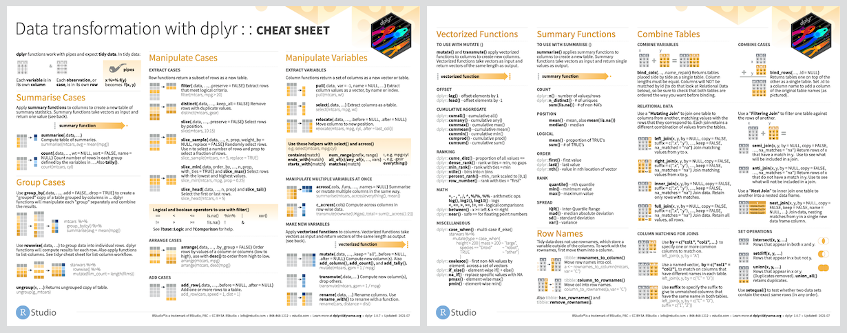
### Data transformation helps you get the data in exactly the right form you need. <br/> With `dplyr` you can:
- create new variables
- create summaries
- rename variables
- reorder observations
- ...and more!
]
.pull-right[
- Pick observations by their values with `filter()`.
- Reorder the rows with `arrange()`.
- Pick variables by their names `select()`.
- Create new variables with functions of existing variables with `mutate()`.
- Collapse many values down to a single summary with `summarize()`.
- `group_by()` gets the above functions to operate group-by-group rather than on the entire dataset.
- and `count()` + `add_count()` simplify `group_by()` + `summarize()` when you just want to count
]
]
.panel[.panel-name[Cheatsheet]
`r icon::fa("file-pdf")` PDF: https://github.com/rstudio/cheatsheets/raw/master/data-transformation.pdf

]
.panel[.panel-name[Reading]
.left-column[
```{r echo=FALSE}
knitr::include_graphics("images/r4ds-cover.png")
```
]
.right-column[
### R for Data Science: [Ch 11 Data transformation](https://r4ds.had.co.nz/transform.html)
### Package documentation: https://dplyr.tidyverse.org/
]
]
]
---
background-image: url(images/hex/dplyr.png)
background-position: 1050px 50px
background-size: 80px
# dplyr: exercise
.panelset[
.panel[.panel-name[Select]
.center[
### Can you spot the difference in performing the same operation?
]
.pull-left[
```{r}
select(penguins, species, sex, body_mass_g)
```
]
.pull-right[
```{r}
penguins %>%
select(species, sex, body_mass_g)
```
]
]
.panel[.panel-name[Arrange]
We can use `arrange()` to arrange our data in descending order by **body_mass_g**
.pull-left[
```{r}
glimpse(penguins)
```
]
.pull-right[
```{r}
penguins %>%
select(species, sex, body_mass_g) %>%
arrange(desc(body_mass_g)) #<<
```
]
]
.panel[.panel-name[Group By & Summarize]
.pull-left[
.middle[We can use `group_by()` to group our data by **species** and **sex**, and `summarize()` to calculate the average **body_mass_g** for each grouping.]
]
.pull-right[
```{r}
penguins %>%
select(species, sex, body_mass_g) %>%
group_by(species, sex) %>% #<<
summarize(mean = mean(body_mass_g)) #<<
```
]
]
.panel[.panel-name[Counting 1]
If we're just interested in _counting_ the observations in each grouping, we can group and summarize with special functions `count()` and `add_count()`.
----
.pull-left[
Counting can be done with `group_by()` and `summarize()`, but it's a little cumbersome.
It involves...
1. using `mutate()` to create an intermediate variable **n_species** that adds up all observations per **species**, and
2. an `ungroup()`-ing step
]
.pull-right[
```{r}
penguins %>%
group_by(species) %>%
mutate(n_species = n()) %>% #<<
ungroup() %>% #<<
group_by(species, sex, n_species) %>%
summarize(n = n())
```
]
]
.panel[.panel-name[Counting 2]
If we're just interested in _counting_ the observations in each grouping, we can group and summarize with special functions `count()` and `add_count()`.
----
.pull-left[
In contrast, `count()` and `add_count()` offer a simplified approach
.small-text[Example kindly [contributed by Alison Hill (@apreshill)](https://github.com/spcanelon/2020-rladies-chi-tidyverse/issues/2)]
]
.pull-right[
```{r}
penguins %>%
count(species, sex) %>%
add_count(species, wt = n, #<<
name = "n_species") #<<
```
]
]
.panel[.panel-name[Mutate]
.pull-left[
We can add to our counting example by using `mutate()` to create a new variable **prop**, which represents the proportion of penguins of each **sex**, grouped by **species**
.small-text[Example kindly [contributed by Alison Hill (@apreshill)](https://github.com/spcanelon/2020-rladies-chi-tidyverse/issues/2)]
]
.pull-right[
```{r}
penguins %>%
count(species, sex) %>%
add_count(species, wt = n,
name = "n_species") %>%
mutate(prop = n/n_species*100) #<<
```
]
]
.panel[.panel-name[Filter]
.pull-left[
Finally, we can filter rows to only show us **Chinstrap** penguin summaries by adding `filter()` to our pipeline]
.pull-right[
```{r}
penguins %>%
count(species, sex) %>%
add_count(species, wt = n,
name = "n_species") %>%
mutate(prop = n/n_species*100) %>%
filter(species == "Chinstrap") #<<
```
]
]
]