Cellular indexing of transcriptomes and epitopes by sequencing (CITE-seq) is a technique that quantifies both gene expression and the abundance of selected surface proteins in each cell simultaneously (Stoeckius et al. 2017).
In this approach, cells are first labelled with antibodies that have been conjugated to synthetic RNA tags. A cell with a higher abundance of a target protein will be bound by more antibodies, causing more molecules of the corresponding antibody-derived tag (ADT) to be attached to that cell. Ref.OSCA
Cell Hashing is based on the exact same principle except that one aims to find a target that's ubiquitously expressed across all cells within the samples. Stoeckius et al., 2018
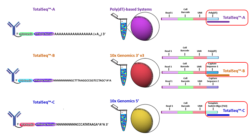
BioLegend supports the protocols with TotalSeq Reagents, i.e. customized antibodies suitable for 10X Genomics' sequencing prep. For the differences between TotalSeq A, B, C see 10X Genomics reply -- in short, their differences have to do with the different sequencing chemistries of different 10X Genomics' protocols.
- How CellRanger handles CITE-seq data
- How to code with CITE-seq data (mostly excerpts from OSCA)
- Hash tags
CellRangerdoesn't explicitly support CITE-seq, but they support generic "antibody capture" results- e.g. dextramers, antigens
- The entries in their
metrics_summary.csvare explained here- e.g.
Antibody: Fraction Antibody Reads in Aggregate Barcodes: Fraction of reads lost after removing aggregate barcodes.
- e.g.
- One specific issue with antibodies are protein aggregates that cause a few GEMs to have extremely high UMI counts.
- "Currently, we consider a barcode an aggregate if it has more than 10K reads, 50% of which were corrected
$" Ref - in addition, "Cell Ranger directly uses protein counts to deduce aggregation events.", i.e. "seeing high counts of many unrelated proteins in a GEM is a sign that such a GEM contains protein aggregates" Ref - if >5 antibodies with min. 1000 counts are detected, GEMs that are in the 25 highest counts across all GEMs will be flagged if the required number of antibodies exceed a pre-deinfed threshold
- a high correction rate is therefore used to flag for protein aggregation
- barcodes with evidence of protein aggregation are removed from the final feature-barcode matrix
- "Currently, we consider a barcode an aggregate if it has more than 10K reads, 50% of which were corrected
- "Antibody aggregation could be triggered by partial unfolding of its domains, leading to monomer-monomer association followed by nucleation and growth. Although the aggregation propensities of antibodies and antibody-based proteins can be affected by the external experimental conditions, they are strongly dependent on the intrinsic antibody properties as determined by their sequences and structures" Li et al., 2016
$CellRanger's UMI correction: Before counting UMIs, Cell Ranger attempts to correct for sequencing errors in the UMI sequences. Reads that were confidently mapped to the transcriptome are placed into groups that share the same barcode, UMI, and gene annotation. If two groups of reads have the same barcode and gene, but their UMIs differ by a single base (i.e., are Hamming distance 1 apart), then one of the UMIs was likely introduced by a substitution error in sequencing. In this case, the UMI of the less-supported read group is corrected to the UMI with higher support. Ref
How should the ADT data be incorporated into the analysis?
-
how 10X measures the antibody levels
-
TotalSeq-C is a line of antibody-oligonucleotide conjugates supplied by BioLegend that are compatible with the Single Cell 5' assay. The Feature Barcode sequence appears at a fixed position (base 10) in the R2 read.
While we have counts for both ADTs and transcripts, there are fundamental differences in nature of the data that make it difficult to treat the former as additional features in the latter:
- small number of antibodies vs. entire transcriptome
- coverage of the ADTs is much deeper (sequencing resources are concentrated into a smaller number of features)
- use of antibodies against protein targets involves consideration of separate biases compared to those observed for transcripts.
from OSCA
from OSCA
# CellRanger data here:
/athena/abc/scratch/paz2005/projects/2020_11_sofia_scrna/cellranger_v5_out
conda create --name citeseq
conda install -c conda-forge r-base
conda install -c conda-forge r-data.table
conda install -c bioconda bioconductor-scuttle
conda install -c bioconda bioconductor-singlecellexperiment
conda install -c r r-ggplot2
SingleCellExperimentclass --> "alternative Experiment"- to store data for different sets of features but the same cells
- can be used to store another SE object inside the SCE object
- often used for spike-in data
- isolates the two sets of features to ensure that analyses on one set o not use data from the other set
sce <- splitAltExps(sce, rowData(sce)$Type)
altExpNames(sce) # Can be used like any other SingleCellExperiment.

# ADT counts are usually not sparse so storage as a sparse matrix provides no advantage
counts(altExp(sce)) <- as.matrix(counts(altExp(sce)))
counts(altExp(sce))[,1:10] # sneak peek
mito <- grep("^MT-", rowData(sce)$Symbol)
df <- perCellQCMetrics(sce, subsets=list(Mito=mito))
mito.discard <- isOutlier(df$subsets_Mito_percent, type="higher")
- remove cells that have failed to capture and/or sequence the ADTs
- background contamination: free antibody or antibody bound to cell fragments
ALL ADTs SHOULD HAVE READS! [otherwise something went wront with the processing!]
# remove cells that have unusually low numbers of detected ADTs
# Applied on the alternative experiment containing the ADT counts:
library(scuttle)
df.ab <- perCellQCMetrics(altExp(sce))

n.nonzero <- sum(!rowAlls(counts(altExp(sce)), value=0L)) # less than or equal to half of the total number of tags
ab.discard <- df.ab$detected <= n.nonzero/2 #
summary(ab.discard)
discard <- ab.discard | mito.discard
sce <- sce[,!discard]
simplest approach is to normalize on the total ADT counts However, ideally, we would like to compute size factors that adjust for the composition biases. This usually requires an assumption that most ADTs are not differentially expressed between cell types/states.
We consider the baseline ADT profile to be a combination of weak constitutive expression and ambient contamination, both of which should be constant across the population. We estimate this profile by assuming that the distribution of abundances for each ADT should be bimodal, where one population of cells exhibits low baseline expression and another population upregulates the corresponding protein target. We then use all cells in the lower mode to compute the baseline abundance for that ADT. This entire calculation is performed by the inferAmbience() function We use a DESeq2-like approach to compute size factors against the baseline profile. Specifically, the size factor for each cell is defined as the median of the ratios of that cell’s counts to the baseline profile. If the abundances for most ADTs in each cell are baseline-derived, they should be roughly constant across cells; any systematic differences in the ratios correspond to cell-specific biases in sequencing coverage and are captured by the size factor. The use of the median protects against the minority of ADTs corresponding to genuinely expressed targets.
baseline <- inferAmbience(counts(altExp(sce)))
# Distribution of (log-)counts for each ADT in the PBMC dataset, with the inferred ambient abundance marked by the black dot.
plotExpression(altExp(sce), features=rownames(altExp(sce)), exprs_values="counts") +
    scale_y_log10() +
    geom_point(data=data.frame(x=names(baseline), y=baseline), mapping=aes(x=x, y=y), cex=3)

sf.amb <- medianSizeFactors(altExp(sce), reference=baseline)
# add median-based size factors to the altExp
sizeFactors(altExp(sce)) <- sf.amb

# logNorm will transform both expression and ADT
sce <- logNormCounts(sce, use.altexps=TRUE)
Unlike transcript-based counts, feature selection is largely unnecessary for analyzing ADT data. This is because feature selection has already occurred during experimental design where the manual choice of target proteins means that all ADTs correspond to interesting features by definition ADT abundances are cleaner (larger counts, stronger signal) for more robust identification of broad cell types
# Set d=NA so that the function does not perform PCA.
g.adt <- buildSNNGraph(altExp(sce), d=NA)
clusters.adt <- igraph::cluster_walktrap(g.adt)$membership

# Generating a t-SNE plot.
library(scater)
set.seed(1010010)
altExp(sce) <- runTSNE(altExp(sce))
colLabels(altExp(sce)) <- factor(clusters.adt)
plotTSNE(altExp(sce), colour_by="label", text_by="label", text_col="red")
If the aim is to test for differences in the functional readout (e.g. using antibodies to target the influenza peptide-MHCII complexes), a natural analysis strategy is to use the transcript data for clustering (Figure 20.13) and perform differential testing between clusters or conditions for the relevant ADTs. The main appeal of this approach is that it avoids data snooping (Section 11.5.1) as the clusters are defined without knowledge of the ADTs. This improves the statistical rigor of the subsequent differential testing on the ADT abundances
From Stoeckius et al., 2018:
HTO raw counts were normalized using centered log ratio (CLR) transformation, where counts were divided by the geometric mean of an HTO across cells and log-transformed
Seurat's HTODemux() function
- k-medoid clustering on normalized HTO values --> cells are separated into K clusters
- "negative" distribution: cluster with lowest average value = negative group for that HTO
- .99 quantile of NB fit used as a threshold to classify cells as positive or negative
- cells with more than one positive HTO call: doublets
OSCA recommends DropletUtils: hashedDrops()
assuming that each HTO has a bimodal distribution where the lower peak corresponds to ambient contamination in cells that do not belong to that HTO’s sample. Counts are then averaged across all cells in the lower mode to obtain the relative abundance of that HTO