A Granular Synthesis playground

The most common definition of sound is related to the concept of wave propagating in space and time. With the emerging developments in the electro-acoustic technologies raised in the XX century, the British physicist Dennis Gabor published in the late 40s three important papers, where he combined theory from quantum mechanics with practical experiment. His idea is that any continuous tone can be decomposed into a family of functions obtained by shifting in time and frequency a single acoustic grain. This theory, strongly affected by psychoacoustics since human hearing is not continuous and infinite in resolution, was born with the publishment by Dr. Ing. D. Gabor of the article "Theory of communication" [1] in which, by the use of the Hilbert Transform and its meaning in the Quantum Mechanical Formalism, he derived a new two-dimensional representation of signals with time and frequency as coordinates which he called "diagram of information": from a complex representation of a signal in time domain, the Hilbert transform of the original signal, and from one in frequency domain derived from Fourier analysis of the Hilbert transform, he created a mathematical abstraction able to map a signal and its energy onto an “effective time and effective spectral width”, calculated as the mean time and frequency of a signal as intended in quantum mechanics, i.e. the value of the operator averaged over the wave function of the system. This is where the Hilbert Transform comes in handy, giving us the possibility to reconstruct the (collapsed) wave function from the real signal and use it to describe signals with the quantum mechanical formalism and also, as we will see, the possibility of applying quantum mechanical transformations to the signal.
Gabor’s analysis can be also thought as a series of localized Fourier transforms.[5]
Gabor also noticed that any analysis requiring signal windowing (such as STFT), entails a strong relationship between time and frequency. High resolution in frequency requires long time windows, at cost of losing track of when exactly some event occurred. Vice versa, having high temporal resolution (short windows), implies losing frequency precision. This strong connection establish a sort of "uncertainty principle", setting the limits of our comprehension of acoustic quanta, and enforcing once again the quantum mechanichal parallelism in his theory.
The main technique on which granular synthesis is based on is granulation, a process in which an audio file is broken down into tiny segments of audio, usually lasting from 5 to 100 ms [[5]]. The sequence of grains in chronological order is called the “graintable”; if grains are played in this order at the speed of the original sample, the output will play back that original file, if one makes sure that amplitude envelopes of overlapping grains sum up to one. If grains are instead played back in a different way (for example by skipping or repeating some of them, by changing their order or applying a frequency shift) different and particular timbres start to emerge.
Because of its eclectic nature, granular synthesis is best used as a textural technique, often for drones, pads, natural sounds and interesting noise layer.
The application is built in C++ using the JUCE framework and an Hilbert transform implementation taken from this software developed by the Harvard-Smithsonian center for astrophysics. It can be used both as a VST3 in a DAW or as a standalone program.
The goal is to provide a useful and relatively simple tool to play with granular synthesis and understand it better, along with easily experiencing independent time-stretching and frequency shifting.
In this section all the controls are explained one by one.

- The audio file can be loaded by pressing the "LOAD" button or by directly dropping it into the screen. Once the file is loaded the waveform is displayed.
- Play/Stop the reproduction.
- Controls the master volume.
- Change the starting position of the granulated section.
- Change the duration of the granulated section. Once the end of the section is reached the reproduction will loop back to the starting position.

As envelope is intended the window applied to each of the grain.
- Display the envelope.
- Select the type of envelope between Gaussian, Trapezoidal and Raised Cosine Bell.
- Change the envelope lobe width.

- Controls how many grains are generated each second. The range goes from 2 to 200 grains per second.
- Controls the duration of the grains. The range goes from 5 ms up to 200 ms.
- Represents the probability of generating a grain from a random position in a range controlled by the "Random Spread" parameter.
- Represents the range in which the randomic grain can be generated.
- Controls the grain scattering speed.

This control is a 2-D canvas in which the user can draw a shape that will control the time (in the original audio file) at which the grains are selected to be played back and their frequency shift. In particular the horizontal axis represents the position of the grain to be selected in the active section, while the vertical axis represents the amount of frequency shift (in Hz) in a range that goes from -2000 Hz to +2000 Hz.
The control is enabled by starting to draw and can be disabled by simply clicking on it.

Display the spectrum of the output signal. The FFT size is of 2048 samples, then it is processed into 256 bins for representation purposes. The vertical line is indicative of the average frequency.

This simple diagram shows the architecture that is behind the implementation.
Following the JUCE structure, there is a PluginProcessor that is in charge of handling the signal processing tasks and a PluginEditor that manages the Graphical User Interface. Upon user interaction the PluginEditor modifies the Model, that is then used in the processor side to retrieve the parameters in real time. Moreover, we decided to add a Granulator class that manages the main granulation algorithm in order to keep it separate and more manageable. In particular, the algorithm dinamically generates the grains according to the parameters retrieved from the Model in real time and deletes them once they have been played. The grains have access to the source file so that they can access the portion that they will contain and can apply the selected envelope to it.
Gabor's ideas connect the quantum mechanichal formalism with the signal theory world. More specifically, all the concepts deriving from the usage of quadrature signals find their explanation in the quantum world parallelism.
A very well done introductory article about quadrature signals is found in [3]; what we will particularly see in this section is how frequency shifting done via a Hilbert Transformer [4] is nothing else than a representation of the quantum mechanichal frequency shift operator and consequently wonder about the families of quantum mechanichal transformations that can be achieved using Hilbert transformers.
Also, we will give a more straightforward and mathematical interpretation of the frequency shifting operation we're doing, in order to tackle this concept from more viewpoints.
To be clear about the meaning of what we're about to say, we want to stress here that with Hilbert transform we intend the complex sum of the real signal along the real axis with its quadrature one along the complex axis H(t) = s(t) + j * a(t) with a(t) being the quadrature signal of s(t). We will not care about if the quadrature signal is the +90 degrees or -90 degrees phase shift version of the original one, being the formalism about taking the real part of the complex signal, operation invariant for complex conjugation.
Starting from the last interpretation mentioned, we understand from [3] how the Hilbert transform represents a complex vector evolving in time in such a way that its real part at any moment represents the real signal at that moment. The following figure represents the Hilbert transform of a sinusoid:
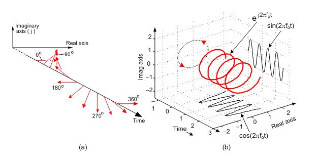
as we can see, this vector rotates in the complex plane as time passes. On to the frequency shifting operation, we understand from [4] that the shifted signal is obtained multiplying the Hilbert transform with exp(j * w * t) with w being the desired shift and t the time passed (mod(2 * PI) to handle phase). Mathematically we know from complex numbers theory that multiplying a complex number with another complex number of unitary module we obtain a rotation of the original number by the phase of the unitary vector or, equivalently, we could say that we are describing the complex number in a reference frame rotated by the phase of the unitary number. So we can now understand better what happens whrn we multiply the Hilbert transform with exp(j * w * t): we can think of this operation as if we are describing the Hilbert transform in a reference frame with the time axis coincident with the one of the previous figure, but with now a complex plane rotating along the time axis with angular velocity w. So, the period of the Hilbert Transform will consequently be lengthened or shortened, depending on the sign of w, by w and consequently the frequency (1 / period) will be modified, resulting in a frequency shift of the Hilbert transform that will of course translate in a frequency shift of its real part, our original signal.
Now that we understand mathematically what is happening, we can move forward and take a look at this operation from a quantum mechanichal point of view. We will assume background knowledge of quantum mechanics and of theory of groups and representations in this explanation, we otherwise suggest to skip to the "Conclusions" section. Our knowledge comes from one of our members which is very happy to be able to suggest for those who want to tackle these concepts references [7] and [8] (any textbook on quantum mechanichs/group theory should anyway be fine).
We know at this point that, from a quantum mechanichal point of view, exp(j * w * t) is a representation of the frequency shift operator and we are applying it on the Hilbert transform of our input signal. Taking the real part of the output of this operation, we obtain our input signal with its spectrum shifted in frequency of the desired amount. We can at the very least say that the fact being of the frequency shift operation having exactly the structure of the quantum shift operator when applied to the Hilbert transform of our real signals, is suspicious. Expecially having knowledge of Gabor's article [1], where this parallelism within signal theory and the quantum mechanichs formalism is so well-exposed. It naturally follows asking ourselves two things:
What does the Hilbert transform of our signal represent from a quantum mechanical point of view?
What quantum transformations can we apply to our signal using this parallelism?
Trying with our (limited) knowledge to answer to these question, starting from the first, as Gabor brillantly explains in [1] the parallelism is all about taking the real part of the quantistic wave function, and what we observe in our "real" world is the collapsed wave function, this last one derived as an eigenfunction of the Hamiltonian operator of the system we are considering as it is represented in our choice of variables used to describe the quantum phase space. Summing up, what we are stating here is that the Hilbert transform of our input signal represents the quantum collapsed wave function. If this is the case, the analytical signal to be a conjugate variable should have, if our input signal is a voltage, dimensions of charge multiplied time [q * t], for the products of the two variables to be an action. We don't have the knowledge about if this is really the case and didn't have enough time to research about it in the time-lapse in which we made this application, anyway what we can say is that everything would be more and more suspicious if the representation of the frequency shift operator with this choice of variables would be the rotation matrix of angle w * t, operation that we applied to our Hilbert Transform to get the frequency shift following [4]. We are not sure about if what we are saying here is new or already known, but if the first is the case we are putting this out here hoping that someone with a deeper grasp of quantum mechanics clears everything out. Some of us (Jacopo Piccirillo) will further research in this direction also.
To the second question, we understand from [9] the importance of canonical transformations and would suggest the subset of physical equivalent transformations to be the family of operations we are wondering about. About audio in particular, we probably would have to restrict ourselves some more to the transformations of the phase space into itself, to get coherent audio data out of audio input.
Getting to practical applications: to get the desired operator, if we are correct, we would need just to compute its representation with Voltage/charge * time as variables as Quantum Mechanics teaches us to do; done that we would have the operator ready to be applied to our Hilbert transform of the input signal. Taking the real part of the output we would have our input transformed according to the selected operation.
In conclusion, we started from the development of a granular synthetyzer and we ended up wandering on Gabor's Parallelism, succeeding in developing a tool exploiting this formalism and getting new doubts, ideas and understanding of Hilbert Transforms and analytical signals, which maybe (unfortunately we didn't have the time still to verify these ideas) could translate in new ways to represent operations on signals in the digital domain derived from Gabor's formalism. All this leading to new tools (as this granular synthetizer) to experience the impact of a quantum formalism on our everyday world, and with quantum mechanics being so hard to grasp also for the difficulty of experiencing it, this would come in quite handy.
Further researchs about this will surely be done, if they have not been made already.
Jacopo Piccirillo
Davide De Marco
Gabriele Stucchi
Matteo Amerena
[1] Theory of Communication, D.Gabor,
[2] Generation and Combination of Grains for Music Synthesis, Douglas L. Jones and Thomas W. Parks
[3] A quadrature signals tutorial: complex, but not complicated, Rick Lyons
[4] Phase or frequency shifting using a Hilbert transformer, Neil Robertson
[5] Microsound, Curtis Roads, MIT Press, 2002
[6] The Basics of Granular Synthesis, Griffin Brown
[7] Principles of Quantum Mechanics, Pauli A. M. Dirac
[8] Group theory and its applications to quantum mechanics of atomic spectra, Eugene P. Wigner
[9] Canonical Transformations in Quantum Mechanics, Arlen Anderson
This project was developed for the course of Sound Analysis Synthesis and Processing (SASP) held by Professor Augusto Sarti at the Politecnico of Milan.