generated from jtr13/bookdown-template
-
Notifications
You must be signed in to change notification settings - Fork 0
/
index.Rmd
413 lines (320 loc) · 21.4 KB
/
index.Rmd
1
2
3
4
5
6
7
8
9
10
11
12
13
14
15
16
17
18
19
20
21
22
23
24
25
26
27
28
29
30
31
32
33
34
35
36
37
38
39
40
41
42
43
44
45
46
47
48
49
50
51
52
53
54
55
56
57
58
59
60
61
62
63
64
65
66
67
68
69
70
71
72
73
74
75
76
77
78
79
80
81
82
83
84
85
86
87
88
89
90
91
92
93
94
95
96
97
98
99
100
101
102
103
104
105
106
107
108
109
110
111
112
113
114
115
116
117
118
119
120
121
122
123
124
125
126
127
128
129
130
131
132
133
134
135
136
137
138
139
140
141
142
143
144
145
146
147
148
149
150
151
152
153
154
155
156
157
158
159
160
161
162
163
164
165
166
167
168
169
170
171
172
173
174
175
176
177
178
179
180
181
182
183
184
185
186
187
188
189
190
191
192
193
194
195
196
197
198
199
200
201
202
203
204
205
206
207
208
209
210
211
212
213
214
215
216
217
218
219
220
221
222
223
224
225
226
227
228
229
230
231
232
233
234
235
236
237
238
239
240
241
242
243
244
245
246
247
248
249
250
251
252
253
254
255
256
257
258
259
260
261
262
263
264
265
266
267
268
269
270
271
272
273
274
275
276
277
278
279
280
281
282
283
284
285
286
287
288
289
290
291
292
293
294
295
296
297
298
299
300
301
302
303
304
305
306
307
308
309
310
311
312
313
314
315
316
317
318
319
320
321
322
323
324
325
326
327
328
329
330
331
332
333
334
335
336
337
338
339
340
341
342
343
344
345
346
347
348
349
350
351
352
353
354
355
356
357
358
359
360
361
362
363
364
365
366
367
368
369
370
371
372
373
374
375
376
377
378
379
380
381
382
383
384
385
386
387
388
389
390
391
392
393
394
395
396
397
398
399
400
401
402
403
404
405
406
407
408
409
410
411
412
413
---
title: "Introducción a RNA-Seq LCG-2021 | Proyecto Final"
author: "Elizabeth Márquez Gómez"
date: "2021-03-01"
site: bookdown::bookdown_site
---
# Introducción
El siguiente proyecto tiene por objetivo aplicar los conocimientos aprendidos en el [curso RNA-seq 2021](https://github.com/lcolladotor/rnaseq_LCG-UNAM_2021). Primer módulo del programa de bioinformática en la Licenciatura en Ciencias Genómicas, Universidad Nacional Autónoma de México.
Por medio de una búsqueda exhaustiva en el paquete [***recount3***](http://bioconductor.org/packages/release/bioc/html/recount3.html) de [***Bioconductor***](http://bioconductor.org/), se identificó el proyecto [***SRP162774 - Variability in the Analgesic Response to Ibuprofen Following Third Molar Extraction is Associated with Differences in Activation of the Cyclooxygenase Pathway***](https://www.biorxiv.org/content/10.1101/467407v1.full), el cuál me pareció adecuado para el análisis de sus datos.
### Abstract del proyecto
*It has long been recognized that there is substantial inter-individual variability in the analgesic efficacy of non-steroidal anti-inflammatory drugs (NSAIDs), but the mechanisms underlying this variability are not well understood. In order to characterize the factors associated with heterogeneity in response to ibuprofen, we performed functional neuroimaging, pharmacokinetic/pharmacodynamic assessments, biochemical assays, and gene expression analysis in twenty-nine healthy subjects who underwent third molar extraction. Subjects were treated with rapid-acting ibuprofen (400 mg; N=19) or placebo (N=10) in a randomized, double-blind design. Compared to placebo, ibuprofen-treated subjects exhibited greater reduction in pain scores, alterations in CBF in brain regions associated with pain processing, and inhibition of ex vivo COX-1 and COX-2 activity and urinary prostaglandin metabolites (p<0.05). Ibuprofen-treated subjects could be stratified into partial responders (N=9, required rescue medication) and complete responders (N=10, no rescue medication). This variability in analgesic efficacy was not associated with demographic/clinical characteristics, markers of systemic inflammation, or ibuprofen pharmacokinetics. Complete responders exhibited less suppression of urinary prostaglandin metabolites and greater induction of serum tumor necrosis factor-a and interleukin 8, compared to partial responders (p<0.05). Partial responders exhibited more alterations in gene expression in peripheral blood mononuclear cells after surgery, with an enrichment in inflammatory pathways. These findings suggest that activation of the prostanoid biosynthetic pathway and regulation of the inflammatory response to surgery differs between partial and complete responders. Future studies are necessary to elucidate the molecular mechanisms underlying this variability and identify biomarkers that are predictive of ibuprofen response. Overall design: Human subjects were given Ibuprofen (400 mg; n=19) or placebo (n=10) following surgical extraction of their third molars. Subjects given Ibuprofen were retrospectively classified as partial responders (n=9) if they required rescue medication (hydrocodone 5 mg/acetaminophen 325 mg), or full responders (n=10) if they did not. All subjects in the placebo group received rescue medication. Blood was collected from subjects before surgery (baseline) and at two time points following surgery (post-surgery 1, post-surgery 2). Both post-surgery samples were collected after subjects were given drug/placebo. Peripheral blood mononuclear cell (PBMCs) were isolated from blood samples and their RNA content was assayed via RNA-seq. The following samples were dropped from normalization and final analyses due to low read depths: GSM3405457 (1004_post-surgery_1), GSM3405459 (1005_post-surgery_1), GSM3405462 (1007_baseline), GSM3405463 (1007_post-surgery_1), GSM3405464 (1008_baseline), GSM3405465 (1008_post-surgery_1), GSM3405466 (1008_post-surgery_2), GSM3405468 (1011_post-surgery_1), GSM3405469 (1011_post-surgery_2), GSM3405472 (1012_post-surgery_2), GSM3405491 (1020_baseline).*
# Importación de datos y carga de bibliotecas
## Descarga de bibliotecas
```{r DownloadingLibraries, message=FALSE, warning=FALSE}
## Cargar el paquete de recount3
library("recount3")
library("edgeR") # BiocManager::install("edgeR", update = FALSE)
library("ggplot2")
library("limma")
library("pheatmap")
library("RColorBrewer")
## Obtener todos los proyectos disponibles de recount3
human_projects <- available_projects()
```
## Importación de datos y evaluación del objeto
```{r creatingObject, message=FALSE, warning=FALSE}
## Descargar el proyecto SRP162774 - Variability in the Analgesic Response to Ibuprofen Following Third Molar Extraction is Associated with Differences in Activation of the Cyclooxygenase Pathway
proj_info <- subset(
human_projects,
project == "SRP162774" & project_type == "data_sources"
)
## Crea un objeto de clase RangedSummarizedExperiment (RSE) con la información a nivel de genes
rse_gene_SRP162774 <- create_rse(proj_info)
```
```{r viewObject}
rse_gene_SRP162774
```
El objeto es analizado con el fin de conocer las categoría que contiene, y evaluar la homogeneidad de las mismas. Si existe algún problema tendrá que ser arreglado por medio de la curación o limpieza de los datos.
```{r evaluatingObject}
## Conversión de las cuentas por nucleotido a cuentas por lectura
assay(rse_gene_SRP162774, "counts") <- compute_read_counts(rse_gene_SRP162774)
##Obtener un resumen más completo sobre el objeto
rse_gene_SRP162774 <- expand_sra_attributes(rse_gene_SRP162774)
colData(rse_gene_SRP162774)[
,
grepl("^sra_attribute", colnames(colData(rse_gene_SRP162774)))
]
```
Al observar una buena integridad de los datos en el paso anterior, no será necesario hacer una limpieza de ellos.
Para el análisis de expresión diferencial, se utilizarán dos atributos del objeto ***drug_treatment*** y ***gender***, ambos pueden ser manejados como *dummy variables*.
```{r viewCharacteristics}
##Verificar los valores de las características a evaluar.
table(rse_gene_SRP162774$sra_attribute.drug_treatment)
table(rse_gene_SRP162774$sra_attribute.gender)
```
# Formateo de datos
Converitir a *factor* los valores a utilizar para el análisis estadístico.
```{r toFactor}
## Convertir a factor las categorías que puedan ser dummy variables
rse_gene_SRP162774$sra_attribute.drug_treatment <- factor(ifelse(rse_gene_SRP162774$sra_attribute.drug_treatment == 'Placebo', 'Placebo', 'Ibuprofen'))
rse_gene_SRP162774$sra_attribute.gender <- factor(rse_gene_SRP162774$sra_attribute.gender)
## Resumen de las variables de interés
summary(as.data.frame(colData(rse_gene_SRP162774)[
,
grepl("^sra_attribute.[cell_line|source_name|treatment]", colnames(colData(rse_gene_SRP162774)))
]))
```
# Transformación de los datos
Ahora se procederá a filtrar y manipular los datos con el fin de obtener los resultados más confiables posibles.
A partir del análisis estadístico de la proporción génica, se puede observar que los valores divergen por una unidad y media aproximadamente, como máximo.
```{r geneProportion}
## Generar la variable que almacena la proporción génica
rse_gene_SRP162774$assigned_gene_prop <- rse_gene_SRP162774$recount_qc.gene_fc_count_all.assigned / rse_gene_SRP162774$recount_qc.gene_fc_count_all.total
summary(rse_gene_SRP162774$assigned_gene_prop)
```
## Filtrado
Para el filtrado de los datos se aplicarán dos parámetros:
- **Calidad de biblioteca**: referente a la proporción de lecturas asignadas a genes sobre las lecturas totales.
- **Nivel de expresión**: basándose en niveles promedio de expresión de los datos y valores como el cpm *(counts per million)*.
```{r statisticData}
## Observar la tendencia de expresión e información estadística de los estados de la categoría a evaluar
with(colData(rse_gene_SRP162774), tapply(assigned_gene_prop, sra_attribute.drug_treatment, summary))
```
A partir del siguiente histograma, es posible observar que la calidad de los datos varía mucho, lo que indica baja calidad de la biblioteca. Sin embargo, se ha decidido proceder con el filtrado y limpieza de datos.
Se decidió que la proporción de muestras sea mayor 0.1, debido la baja frecuencia de aquellas previas al corte 0.1. Debe resaltarse, que aún así siguen existiendo algunas muestras con baja, pero se intentó perder la menor información posible. Esto también se basa en las proporciones observadas anteriormente, donde el primer cuartil de ambos estados es ~0.1 por lo que podemos tomarlo como punto de corte.
Para la parte de la cola (derecha), a pesar de tener baja frecuencia, son datos más confiables, por lo cual no se eliminaron.
```{r}
## Salvar información cruda del proyecto
rse_gene_SRP162774_unfiltered <- rse_gene_SRP162774
## Eliminar muestras malas
colorGradient <- colorRampPalette(c('gold','firebrick1'))
hist(rse_gene_SRP162774$assigned_gene_prop, col = colorGradient(20), main='Distribución de expresión génica en rse_gene_SRP162774', xlab='Expresión', ylab='Frecuencia')
abline(v = 0.1, col="dodgerblue3", lwd=3, lty=2)
## Verificar el número de muestras que cumplen con el criterio
table(rse_gene_SRP162774$assigned_gene_prop < 0.1)
```
Aplicar el corte al pico de la distribución. Se observa una forma más aceptable.
A partir del análisis estadístico, se decidirá el valor mínimo para la calidad de expresión génica. Ya que el mínimo y el primer cuartil presentan 0.000, y la media tiene un valor muy bajo aún. Se tomará como punto de corte a 0.1 (muestras poco informativas)
```{r cutoff1}
## Realizar el corte y observar la distribución
rse_gene_SRP162774 <- rse_gene_SRP162774[, rse_gene_SRP162774$assigned_gene_prop > 0.1]
colorGradient <- colorRampPalette(c('darkslategray1','dodgerblue4'))
hist(rse_gene_SRP162774$assigned_gene_prop, col = colorGradient(13), main='Distribución de expresión génica en rse_gene_SRP162774 con cutoff', xlab='Expresión', ylab='Frecuencia')
abline(v = 0.1, col="red", lwd=3, lty=2)
## Se calculan los niveles medios de expresión de los genes en las muestras
gene_means <- rowMeans(assay(rse_gene_SRP162774, "counts"))
summary(gene_means)
```
Debido a los resultados del análisis estadístico anterior, donde el 1er cuartil y la media toman valores de 0, se procederá a tomar 0.1 como valor mínimo para niveles de expresión génica.
```{r cutoff2}
## Eliminar genes con menor a 0.1
rse_gene_SRP162774 <- rse_gene_SRP162774[gene_means > 0.1, ]
## Comparar dimensión final
dim(rse_gene_SRP162774_unfiltered)
dim(rse_gene_SRP162774)
```
Después de la limpieza, se ha conservado el 41.73% del total de los datos. La gran pérdida de los mismos se atribuye a una baja caliad de la biblioteca original.
```{r conservationPercentage}
#Obtener el porcentaje de información conservada después de la limpieza
round(nrow(rse_gene_SRP162774) / nrow(rse_gene_SRP162774_unfiltered) * 100, 2)
```
Se decidió probar con limpieza automatizada por medio de la función *keep.exprs* de ***limma*** con la esperanza de obtener una integridad mayor de los datos.
```{r normalizationAuto }
#Calculo de factores de normalización
dge_auto <- DGEList(
counts = assay(rse_gene_SRP162774, "counts"),
genes = rowData(rse_gene_SRP162774)
)
dge_auto <- calcNormFactors(dge_auto)
```
```{r createCPM}
cpm <- cpm(dge_auto)
lcpm <- cpm(dge_auto, log=TRUE)
L <- mean(dge_auto$samples$lib.size) * 1e-6
M <- median(dge_auto$samples$lib.size) * 1e-6
c(L, M)
```
```{r keep}
## Determinarémos cuáles genes cuentan con un nivel de expresión significativo con la función filterByExpr.
keep.exprs <- filterByExpr(dge_auto, group=dge_auto$samples$group)
dge_auto <- dge_auto[keep.exprs,, keep.lib.sizes=FALSE]
dim(dge_auto)
dim(rse_gene_SRP162774)
```
El filtrado automatizado logró conservar el 12.49% de los datos. Por esto mismo se decidió no proceder con esta información, ya que es muy poca.
```{r percentageAuto}
round(nrow(dge_auto) / nrow(rse_gene_SRP162774) * 100, 2)
```
El siguiente gráfico muestra el corte de datos realizado por *keep.exprs* debido a su baja calidad.
```{r comparison}
lcpm.cutoff <- log2(10/M + 2/L)
nsamples <- ncol(dge_auto)
col <- brewer.pal(nsamples, "Paired")
par(mfrow=c(1,2))
plot(density(lcpm[,1]), col=col[1], lwd=2, las=2, main="", xlab="")
title(main="A. Raw data", xlab="Log-cpm")
abline(v=lcpm.cutoff, lty=3)
for (i in 2:nsamples){
den <- density(lcpm[,i])
lines(den$x, den$y, col=col[i], lwd=2)
}
lcpm <- cpm(dge_auto, log=TRUE)
plot(density(lcpm[,1]), col=col[1], lwd=2, las=2, main="", xlab="")
title(main="B. Filtered data", xlab="Log-cpm")
abline(v=lcpm.cutoff, lty=3)
for (i in 2:nsamples){
den <- density(lcpm[,i])
lines(den$x, den$y, col=col[i], lwd=2)
}
```
# Visualización
Se procederá al análisis visual de los datos ya curados y normalizados. Se evaluarán las dos categorías indicativas del objeto "sexo" y "tratamiento"
```{r normalization}
#Calculo de factores de normalización
dge <- DGEList(
counts = assay(rse_gene_SRP162774, "counts"),
genes = rowData(rse_gene_SRP162774)
)
dge <- calcNormFactors(dge)
```
La siguiente gráfica ilustra la distribución de expresión de ambas condiciones. Por lo que se puede ver que están encasilladas entre 0.1 a poco más de 0.21, ambas condiciones tienen expresión similar, sin embargo se puede percibir un grupo de *outliers* para la expresión de ibuprofeno
```{r boxPlotExpression1}
## Visualización de expresión por medio de boxplot
ggplot(as.data.frame(colData(rse_gene_SRP162774)), aes(y = assigned_gene_prop, x = sra_attribute.drug_treatment, fill=sra_attribute.drug_treatment)) +
geom_boxplot(alpha=0.3) +
theme_bw(base_size = 20) +
ylab("Proporción génica") +
xlab("Tratamiento") +
theme(legend.position="top", legend.title = element_text(size = 13), legend.text = element_text(size = 8)) +
labs(fill = "Relación de expresión génica con tipo de tratamiento |")
```
```{r boxPlotExpression2}
ggplot(as.data.frame(colData(rse_gene_SRP162774)), aes(y = assigned_gene_prop, x = sra_attribute.gender, fill=sra_attribute.gender)) +
geom_boxplot(alpha=0.3) +
theme_bw(base_size = 20) +
ylab("Proporción génica") +
xlab("Sexo") +
theme(legend.position="top", legend.title = element_text(size = 13), legend.text = element_text(size = 8)) +
labs(fill = "Relación de expresión génica con sexo |")
```
# Modelado estadístico
Se usará `model.matrix()` para modelar las dos categorías para el análisis de expresión diferencial.
```{r getVariablesOrder}
mod <- model.matrix(~ sra_attribute.drug_treatment + sra_attribute.gender + assigned_gene_prop,
data = colData(rse_gene_SRP162774)
)
colnames(mod)
```
```{r validateDummyVariables}
## Verificar las posiciones de 1 y 0 respecto al estado de la categoría
head(rse_gene_SRP162774$sra_attribute.drug_treatment)
head(mod)
print(rse_gene_SRP162774$sra_attribute.drug_treatment[17])
print(mod[17])
```
La siguiente gráfica ilustra el promedio de varianza en la expresión diferencial de los datos. A partir de esto podemos observar el aunque se ajustan al promedio, la desviación se elonga aproximadamente 0.8 unidades. Es necesario acercar a los genes lejanos a la línea roja.
```{r voom}
vGene <- voom(dge, mod, plot = TRUE)
```
A partir de lo anterior, es necesario generar un modelo de regresión lineal para ajustar la expresión de los datos.Obtención del p-value por medio de la función eBayes.
```{r pValue}
eb_results <- eBayes(lmFit(vGene))
## Se configura el coef en 2, ya que ahí se encuentra la variable a evaluar (de referencia)
de_results <- topTable(
eb_results,
coef = 2,
number = nrow(rse_gene_SRP162774),
sort.by = "none"
)
dim(de_results)
```
```{r view2}
head(de_results)
```
Evaluar p-value menor a 0.05
```{r evaluatePValue}
## Genes diferencialmente expresados entre ibuprofeno y placebo con FDR < 5%
table(de_results$adj.P.Val < 0.05)
```
La siguiente gráfica explica el cambio de expresión entre placebo e ibupofeno. Los valores positivos indican una expresión más alta en placebo y valores negativos indican mayor expresión en ibuprofeno.
```{r viewStatisticResults}
## Visualizar resultados estadísticos
plotMA(eb_results, coef = 2)
abline(h = 0.25, col="red", lwd=3, lty=2)
abline(h = -0.25, col="red", lwd=3, lty=2)
```
El gráfico siguiente ilustra el *logfold change* en el eje x y el *p-value* en el eje y. Esto permite dilucidar los genes con mayor expresión y con mejor valor de *p-value*.
Los 3 genes con mayor expresión se resaltan en azul.
```{r mostExpressed}
#Checar los genes en genecards
volcanoplot(eb_results, coef = 2, highlight = 3, names = de_results$gene_name)
```
El el siguiente heatmap podemos observar algunas clusterizaciones intermitentes para la clasificación de sexo. En la clasificación de tratamiento se observan un más grandes, lo que indica una buena relación en los datos. Respecto a los genes, sí es posible ver clusterización en relación a su nivel de expresión.
```{r}
## Extracción de valores de genes de interés
exprs_heatmap <- vGene$E[rank(de_results$adj.P.Val) <= 50, ]
## Crear una tabla con información de las muestras
df <- as.data.frame(colData(rse_gene_SRP162774)[, c("sra_attribute.drug_treatment", "sra_attribute.gender")])
colnames(df) <- c("treatment", "gender")
## Cambiar ID a nombre de los genes
rownames(exprs_heatmap)
findPositions <- which(rowRanges(rse_gene_SRP162774)$gene_id %in% rownames(exprs_heatmap))
rownames(exprs_heatmap) <- rowRanges(rse_gene_SRP162774)$gene_name[findPositions]
pheatmap(
exprs_heatmap,
cluster_rows = TRUE,
cluster_cols = TRUE,
show_rownames = TRUE,
show_colnames = FALSE,
annotation_col = df,
fontsize_row = 4
)
```
```{r}
## Para colores
head(df)
## Conviertiendo los grupos de tratamiento a colores
col.drug <- df$treatment
levels(col.drug) <- brewer.pal(nlevels(col.drug), "Set1")
```
A pesar de la limpieza realizada a los datos, no es posible observar una clusterización referente al tipo de tratamiento en los niveles de expresión. Lo anterior, puede atribuirse a una baja calidad de la biblioteca de datos o a un nivel de expresión realmente bajo en ambas condiciones.
```{r}
col.drug <- as.character(col.drug)
## MDS por grupos tratamiento
plotMDS(vGene$E, labels = df$treatment, col = col.drug)
```
Los siguientes gráficos sugieren una alta relación entre la respuesta a ibuprofeno ligada a los hombres, y la respuesta a placebo ligada a las mujeres. Sin embargo la clusterización no es tan clara para afirmar esta hipótesis.
```{r}
## Conviertiendo los grupos de tratamiento a colores
col.sex <- df$gender
levels(col.sex) <- brewer.pal(nlevels(col.sex), "Dark2")
col.sex <- as.character(col.sex)
## MDS por grupos tratamiento
plotMDS(vGene$E, labels = df$gender, col = col.sex)
```
```{r}
plot(df, main = 'Relación entre sexo y tipo de tratamiento', col = c('darkseagreen1', 'lightblue'))
```
# Interpretación
Finalmente, es importante recalcar la importancia de la buena calidad de las bibliotecas de datos para un análisis de expresión diferencial adecuado. Tristemente no fue posible hacer una gran evaluación debido a la alta pérdida de datos y baja expresión diferencial del proyecto.
Los datos fueron sometidos a un proceso de análisis, limpieza, manipulación, modelaje, visualización e interpretración establecido por: 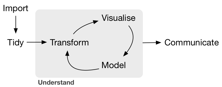
Esto con el fin de purificar la biblioteca de datos y obtener la mejor calidad posible para su análisis.
Algunos de los retos que se presentaron fue el bajo número de características a usar para el análisis. Así como la definición adecuada de los puntos de corte que permitieran mejorar la calidad de los datos, pero al mismo tiempo evitar una pérdida masiva de los mismos.
A pesar de los resultados obtenidos en este proyecto, creo que realizarlo fue una excelente oportunidad como el primer acercamiento a la bioinformática. Y los conocimientos adquiridos han sido de mucha utilidad como los primeros pasos de futuros proyectos más elaborados. Deseo que en un futuro tenga la oportunidad de desarrollarme más en esta área de la bioinformática y descubrir más herramientas que permitan análisis más completos y certeros de los datos.
# Autoría y referencias
## Autora
- [Elizabeth Márquez Gómez](https://elizabeth-mqz-gmz.github.io/)
- [Elizabeth GitHub](https://github.com/Elizabeth-mqz-gmz)
## Referencias
- [Curso RNA-seq 2021](https://github.com/lcolladotor/rnaseq_LCG-UNAM_2021)
- [Leonardo Collado-Torres](http://lcolladotor.github.io/)
- Collado-Torres L (2021). Explore and download data from the recount3 project. doi: 10.18129/B9.bioc.recount3 (URL:
https://doi.org/10.18129/B9.bioc.recount3), https://github.com/LieberInstitute/recount3 - R package version 1.0.7, <URL:
http://www.bioconductor.org/packages/recount3>.
- Robinson MD, McCarthy DJ and Smyth GK (2010). edgeR: a Bioconductor package for differential expression analysis of digital gene
expression data. Bioinformatics 26, 139-140
- H. Wickham. ggplot2: Elegant Graphics for Data Analysis. Springer-Verlag New York, 2016.
- Ritchie ME, Phipson B, Wu D, Hu Y, Law CW, Shi W, Smyth GK (2015). “limma powers differential expression analyses for RNA-sequencing and microarray studies.” Nucleic Acids Research, 43(7), e47. doi: 10.1093/nar/gkv007, https://doi.org/10.1093/nar/gkv007
- Kolde, R. (2019). "pheatmap: Pretty Heatmaps." CRAN-r-project, https://CRAN.R-project.org/package=pheatmap
- Neuwirth, E. (2014). "RColorBrewer: ColorBrewer Palettes." CRAN-r-project, https://CRAN.R-project.org/package=RColorBrewer