-
Notifications
You must be signed in to change notification settings - Fork 1
/
Copy path1.3-Model_validation_and_Resampling.html
1242 lines (1134 loc) · 62.7 KB
/
1.3-Model_validation_and_Resampling.html
1
2
3
4
5
6
7
8
9
10
11
12
13
14
15
16
17
18
19
20
21
22
23
24
25
26
27
28
29
30
31
32
33
34
35
36
37
38
39
40
41
42
43
44
45
46
47
48
49
50
51
52
53
54
55
56
57
58
59
60
61
62
63
64
65
66
67
68
69
70
71
72
73
74
75
76
77
78
79
80
81
82
83
84
85
86
87
88
89
90
91
92
93
94
95
96
97
98
99
100
101
102
103
104
105
106
107
108
109
110
111
112
113
114
115
116
117
118
119
120
121
122
123
124
125
126
127
128
129
130
131
132
133
134
135
136
137
138
139
140
141
142
143
144
145
146
147
148
149
150
151
152
153
154
155
156
157
158
159
160
161
162
163
164
165
166
167
168
169
170
171
172
173
174
175
176
177
178
179
180
181
182
183
184
185
186
187
188
189
190
191
192
193
194
195
196
197
198
199
200
201
202
203
204
205
206
207
208
209
210
211
212
213
214
215
216
217
218
219
220
221
222
223
224
225
226
227
228
229
230
231
232
233
234
235
236
237
238
239
240
241
242
243
244
245
246
247
248
249
250
251
252
253
254
255
256
257
258
259
260
261
262
263
264
265
266
267
268
269
270
271
272
273
274
275
276
277
278
279
280
281
282
283
284
285
286
287
288
289
290
291
292
293
294
295
296
297
298
299
300
301
302
303
304
305
306
307
308
309
310
311
312
313
314
315
316
317
318
319
320
321
322
323
324
325
326
327
328
329
330
331
332
333
334
335
336
337
338
339
340
341
342
343
344
345
346
347
348
349
350
351
352
353
354
355
356
357
358
359
360
361
362
363
364
365
366
367
368
369
370
371
372
373
374
375
376
377
378
379
380
381
382
383
384
385
386
387
388
389
390
391
392
393
394
395
396
397
398
399
400
401
402
403
404
405
406
407
408
409
410
411
412
413
414
415
416
417
418
419
420
421
422
423
424
425
426
427
428
429
430
431
432
433
434
435
436
437
438
439
440
441
442
443
444
445
446
447
448
449
450
451
452
453
454
455
456
457
458
459
460
461
462
463
464
465
466
467
468
469
470
471
472
473
474
475
476
477
478
479
480
481
482
483
484
485
486
487
488
489
490
491
492
493
494
495
496
497
498
499
500
501
502
503
504
505
506
507
508
509
510
511
512
513
514
515
516
517
518
519
520
521
522
523
524
525
526
527
528
529
530
531
532
533
534
535
536
537
538
539
540
541
542
543
544
545
546
547
548
549
550
551
552
553
554
555
556
557
558
559
560
561
562
563
564
565
566
567
568
569
570
571
572
573
574
575
576
577
578
579
580
581
582
583
584
585
586
587
588
589
590
591
592
593
594
595
596
597
598
599
600
601
602
603
604
605
606
607
608
609
610
611
612
613
614
615
616
617
618
619
620
621
622
623
624
625
626
627
628
629
630
631
632
633
634
635
636
637
638
639
640
641
642
643
644
645
646
647
648
649
650
651
652
653
654
655
656
657
658
659
660
661
662
663
664
665
666
667
668
669
670
671
672
673
674
675
676
677
678
679
680
681
682
683
684
685
686
687
688
689
690
691
692
693
694
695
696
697
698
699
700
701
702
703
704
705
706
707
708
709
710
711
712
713
714
715
716
717
718
719
720
721
722
723
724
725
726
727
728
729
730
731
732
733
734
735
736
737
738
739
740
741
742
743
744
745
746
747
748
749
750
751
752
753
754
755
756
757
758
759
760
761
762
763
764
765
766
767
768
769
770
771
772
773
774
775
776
777
778
779
780
781
782
783
784
785
786
787
788
789
790
791
792
793
794
795
796
797
798
799
800
801
802
803
804
805
806
807
808
809
810
811
812
813
814
815
816
817
818
819
820
821
822
823
824
825
826
827
828
829
830
831
832
833
834
835
836
837
838
839
840
841
842
843
844
845
846
847
848
849
850
851
852
853
854
855
856
857
858
859
860
861
862
863
864
865
866
867
868
869
870
871
872
873
874
875
876
877
878
879
880
881
882
883
884
885
886
887
888
889
890
891
892
893
894
895
896
897
898
899
900
901
902
903
904
905
906
907
908
909
910
911
912
913
914
915
916
917
918
919
920
921
922
923
924
925
926
927
928
929
930
931
932
933
934
935
936
937
938
939
940
941
942
943
944
945
946
947
948
949
950
951
952
953
954
955
956
957
958
959
960
961
962
963
964
965
966
967
968
969
970
971
972
973
974
975
976
977
978
979
980
981
982
983
984
985
986
987
988
989
990
991
992
993
994
995
996
997
998
999
1000
<!DOCTYPE html>
<html lang="en"><head>
<script src="1.3-Model_validation_and_Resampling_files/libs/clipboard/clipboard.min.js"></script>
<script src="1.3-Model_validation_and_Resampling_files/libs/quarto-html/tabby.min.js"></script>
<script src="1.3-Model_validation_and_Resampling_files/libs/quarto-html/popper.min.js"></script>
<script src="1.3-Model_validation_and_Resampling_files/libs/quarto-html/tippy.umd.min.js"></script>
<link href="1.3-Model_validation_and_Resampling_files/libs/quarto-html/tippy.css" rel="stylesheet">
<link href="1.3-Model_validation_and_Resampling_files/libs/quarto-html/light-border.css" rel="stylesheet">
<link href="1.3-Model_validation_and_Resampling_files/libs/quarto-html/quarto-html.min.css" rel="stylesheet" data-mode="light">
<link href="1.3-Model_validation_and_Resampling_files/libs/quarto-html/quarto-syntax-highlighting.css" rel="stylesheet" id="quarto-text-highlighting-styles"><meta charset="utf-8">
<meta name="generator" content="quarto-1.4.549">
<meta name="author" content="Alex Sanchez, Ferran Reverter and Esteban Vegas">
<title>Model validation and Resampling</title>
<meta name="apple-mobile-web-app-capable" content="yes">
<meta name="apple-mobile-web-app-status-bar-style" content="black-translucent">
<meta name="viewport" content="width=device-width, initial-scale=1.0, maximum-scale=1.0, user-scalable=no, minimal-ui">
<link rel="stylesheet" href="1.3-Model_validation_and_Resampling_files/libs/revealjs/dist/reset.css">
<link rel="stylesheet" href="1.3-Model_validation_and_Resampling_files/libs/revealjs/dist/reveal.css">
<style>
code{white-space: pre-wrap;}
span.smallcaps{font-variant: small-caps;}
div.columns{display: flex; gap: min(4vw, 1.5em);}
div.column{flex: auto; overflow-x: auto;}
div.hanging-indent{margin-left: 1.5em; text-indent: -1.5em;}
ul.task-list{list-style: none;}
ul.task-list li input[type="checkbox"] {
width: 0.8em;
margin: 0 0.8em 0.2em -1em; /* quarto-specific, see https://github.com/quarto-dev/quarto-cli/issues/4556 */
vertical-align: middle;
}
</style>
<link rel="stylesheet" href="1.3-Model_validation_and_Resampling_files/libs/revealjs/dist/theme/quarto.css">
<link rel="stylesheet" href="css4CU.css">
<link href="1.3-Model_validation_and_Resampling_files/libs/revealjs/plugin/quarto-line-highlight/line-highlight.css" rel="stylesheet">
<link href="1.3-Model_validation_and_Resampling_files/libs/revealjs/plugin/reveal-menu/menu.css" rel="stylesheet">
<link href="1.3-Model_validation_and_Resampling_files/libs/revealjs/plugin/reveal-menu/quarto-menu.css" rel="stylesheet">
<link href="1.3-Model_validation_and_Resampling_files/libs/revealjs/plugin/quarto-support/footer.css" rel="stylesheet">
<style type="text/css">
.callout {
margin-top: 1em;
margin-bottom: 1em;
border-radius: .25rem;
}
.callout.callout-style-simple {
padding: 0em 0.5em;
border-left: solid #acacac .3rem;
border-right: solid 1px silver;
border-top: solid 1px silver;
border-bottom: solid 1px silver;
display: flex;
}
.callout.callout-style-default {
border-left: solid #acacac .3rem;
border-right: solid 1px silver;
border-top: solid 1px silver;
border-bottom: solid 1px silver;
}
.callout .callout-body-container {
flex-grow: 1;
}
.callout.callout-style-simple .callout-body {
font-size: 1rem;
font-weight: 400;
}
.callout.callout-style-default .callout-body {
font-size: 0.9rem;
font-weight: 400;
}
.callout.callout-titled.callout-style-simple .callout-body {
margin-top: 0.2em;
}
.callout:not(.callout-titled) .callout-body {
display: flex;
}
.callout:not(.no-icon).callout-titled.callout-style-simple .callout-content {
padding-left: 1.6em;
}
.callout.callout-titled .callout-header {
padding-top: 0.2em;
margin-bottom: -0.2em;
}
.callout.callout-titled .callout-title p {
margin-top: 0.5em;
margin-bottom: 0.5em;
}
.callout.callout-titled.callout-style-simple .callout-content p {
margin-top: 0;
}
.callout.callout-titled.callout-style-default .callout-content p {
margin-top: 0.7em;
}
.callout.callout-style-simple div.callout-title {
border-bottom: none;
font-size: .9rem;
font-weight: 600;
opacity: 75%;
}
.callout.callout-style-default div.callout-title {
border-bottom: none;
font-weight: 600;
opacity: 85%;
font-size: 0.9rem;
padding-left: 0.5em;
padding-right: 0.5em;
}
.callout.callout-style-default div.callout-content {
padding-left: 0.5em;
padding-right: 0.5em;
}
.callout.callout-style-simple .callout-icon::before {
height: 1rem;
width: 1rem;
display: inline-block;
content: "";
background-repeat: no-repeat;
background-size: 1rem 1rem;
}
.callout.callout-style-default .callout-icon::before {
height: 0.9rem;
width: 0.9rem;
display: inline-block;
content: "";
background-repeat: no-repeat;
background-size: 0.9rem 0.9rem;
}
.callout-title {
display: flex
}
.callout-icon::before {
margin-top: 1rem;
padding-right: .5rem;
}
.callout.no-icon::before {
display: none !important;
}
.callout.callout-titled .callout-body > .callout-content > :last-child {
padding-bottom: 0.5rem;
margin-bottom: 0;
}
.callout.callout-titled .callout-icon::before {
margin-top: .5rem;
padding-right: .5rem;
}
.callout:not(.callout-titled) .callout-icon::before {
margin-top: 1rem;
padding-right: .5rem;
}
/* Callout Types */
div.callout-note {
border-left-color: #4582ec !important;
}
div.callout-note .callout-icon::before {
background-image: url('data:image/png;base64,iVBORw0KGgoAAAANSUhEUgAAACAAAAAgCAYAAABzenr0AAAAAXNSR0IArs4c6QAAAERlWElmTU0AKgAAAAgAAYdpAAQAAAABAAAAGgAAAAAAA6ABAAMAAAABAAEAAKACAAQAAAABAAAAIKADAAQAAAABAAAAIAAAAACshmLzAAAEU0lEQVRYCcVXTWhcVRQ+586kSUMMxkyaElstCto2SIhitS5Ek8xUKV2poatCcVHtUlFQk8mbaaziwpWgglJwVaquitBOfhQXFlqlzSJpFSpIYyXNjBNiTCck7x2/8/LeNDOZxDuEkgOXe++553zfefee+/OYLOXFk3+1LLrRdiO81yNqZ6K9cG0P3MeFaMIQjXssE8Z1JzLO9ls20MBZX7oG8w9GxB0goaPrW5aNMp1yOZIa7Wv6o2ykpLtmAPs/vrG14Z+6d4jpbSKuhdcSyq9wGMPXjonwmESXrriLzFGOdDBLB8Y6MNYBu0dRokSygMA/mrun8MGFN3behm6VVAwg4WR3i6FvYK1T7MHo9BK7ydH+1uurECoouk5MPRyVSBrBHMYwVobG2aOXM07sWrn5qgB60rc6mcwIDJtQrnrEr44kmy+UO9r0u9O5/YbkS9juQckLed3DyW2XV/qWBBB3ptvI8EUY3I9p/67OW+g967TNr3Sotn3IuVlfMLVnsBwH4fsnebJvyGm5GeIUA3jljERmrv49SizPYuq+z7c2H/jlGC+Ghhupn/hcapqmcudB9jwJ/3jvnvu6vu5lVzF1fXyZuZZ7U8nRmVzytvT+H3kilYvH09mLWrQdwFSsFEsxFVs5fK7A0g8gMZjbif4ACpKbjv7gNGaD8bUrlk8x+KRflttr22JEMRUbTUwwDQScyzPgedQHZT0xnx7ujw2jfVfExwYHwOsDTjLdJ2ebmeQIlJ7neo41s/DrsL3kl+W2lWvAga0tR3zueGr6GL78M3ifH0rGXrBC2aAR8uYcIA5gwV8zIE8onoh8u0Fca/ciF7j1uOzEnqcIm59sEXoGc0+z6+H45V1CvAvHcD7THztu669cnp+L0okAeIc6zjbM/24LgGM1gZk7jnRu1aQWoU9sfUOuhrmtaPIO3YY1KLLWZaEO5TKUbMY5zx8W9UJ6elpLwKXbsaZ4EFl7B4bMtDv0iRipKoDQT2sNQI9b1utXFdYisi+wzZ/ri/1m7QfDgEuvgUUEIJPq3DhX/5DWNqIXDOweC2wvIR90Oq3lDpdMIgD2r0dXvGdsEW5H6x6HLRJYU7C69VefO1x8Gde1ZFSJLfWS1jbCnhtOPxmpfv2LXOA2Xk2tvnwKKPFuZ/oRmwBwqRQDcKNeVQkYcOjtWVBuM/JuYw5b6isojIkYxyYAFn5K7ZBF10fea52y8QltAg6jnMqNHFBmGkQ1j+U43HMi2xMar1Nv0zGsf1s8nUsmUtPOOrbFIR8bHFDMB5zL13Gmr/kGlCkUzedTzzmzsaJXhYawnA3UmARpiYj5ooJZiUoxFRtK3X6pgNPv+IZVPcnwbOl6f+aBaO1CNvPW9n9LmCp01nuSaTRF2YxHqZ8DYQT6WsXT+RD6eUztwYLZ8rM+rcPxamv1VQzFUkzFXvkiVrySGQgJNvXHJAxiU3/NwiC03rSf05VBaPtu/Z7/B8Yn/w7eguloAAAAAElFTkSuQmCC');
}
div.callout-note.callout-style-default .callout-title {
background-color: #dae6fb
}
div.callout-important {
border-left-color: #d9534f !important;
}
div.callout-important .callout-icon::before {
background-image: url('data:image/png;base64,iVBORw0KGgoAAAANSUhEUgAAACAAAAAgCAYAAABzenr0AAAAAXNSR0IArs4c6QAAAERlWElmTU0AKgAAAAgAAYdpAAQAAAABAAAAGgAAAAAAA6ABAAMAAAABAAEAAKACAAQAAAABAAAAIKADAAQAAAABAAAAIAAAAACshmLzAAAEKklEQVRYCcVXTWhcVRS+575MJym48A+hSRFr00ySRQhURRfd2HYjk2SSTokuBCkU2o0LoSKKraKIBTcuFCoidGFD08nkBzdREbpQ1EDNIv8qSGMFUboImMSZd4/f9zJv8ibJMC8xJQfO3HPPPef7zrvvvnvviIkpC9nsw0UttFunbUhpFzFtarSd6WJkStVMw5xyVqYTvkwfzuf/5FgtkVoB0729j1rjXwThS7Vio+Mo6DNnvLfahoZ+i/o32lULuJ3NNiz7q6+pyAUkJaFF6JwaM2lUJlV0MlnQn5aTRbEu0SEqHUa0A4AdiGuB1kFXRfVyg5d87+Dg4DL6m2TLAub60ilj7A1Ec4odSAc8X95sHh7+ZRPCFo6Fnp7HfU/fBng/hi10CjCnWnJjsxvDNxWw0NfV6Rv5GgP3I3jGWXumdTD/3cbEOP2ZbOZp69yniG3FQ9z1jD7bnBu9Fc2tKGC2q+uAJOQHBDRiZX1x36o7fWBs7J9ownbtO+n0/qWkvW7UPIfc37WgT6ZGR++EOJyeQDSb9UB+DZ1G6DdLDzyS+b/kBCYGsYgJbSQHuThGKRcw5xdeQf8YdNHsc6ePXrlSYMBuSIAFTGAtQo+VuALo4BX83N190NWZWbynBjhOHsmNfFWLeL6v+ynsA58zDvvAC8j5PkbOcXCMg2PZFk3q8MjI7WAG/Dp9AwP7jdGBOOQkAvlFUB+irtm16I1Zw9YBcpGTGXYmk3kQIC/Cds55l+iMI3jqhjAuaoe+am2Jw5GT3Nbz3CkE12NavmzN5+erJW7046n/CH1RO/RVa8lBLozXk9uqykkGAyRXLWlLv5jyp4RFsG5vGVzpDLnIjTWgnRy2Rr+tDKvRc7Y8AyZq10jj8DqXdnIRNtFZb+t/ZRtXcDiVnzpqx8mPcDWxgARUqx0W1QB9MeUZiNrV4qP+Ehc+BpNgATsTX8ozYKL2NtFYAHc84fG7ndxUPr+AR/iQSns7uSUufAymwDOb2+NjK27lEFocm/EE2WpyIy/Hi66MWuMKJn8RvxIcj87IM5Vh9663ziW36kR0HNenXuxmfaD8JC7tfKbrhFr7LiZCrMjrzTeGx+PmkosrkNzW94ObzwocJ7A1HokLolY+AvkTiD/q1H0cN48c5EL8Crkttsa/AXQVDmutfyku0E7jShx49XqV3MFK8IryDhYVbj7Sj2P2eBxwcXoe8T8idsKKPRcnZw1b+slFTubwUwhktrfnAt7J++jwQtLZcm3sr9LQrjRzz6cfMv9aLvgmnAGvpoaGLxM4mAEaLV7iAzQ3oU0IvD5x9ix3yF2RAAuYAOO2f7PEFWCXZ4C9Pb2UsgDeVnFSpbFK7/IWu7TPTvBqzbGdCHOJQSxiEjt6IyZmxQyEJHv6xyQsYk//moVFsN2zP6fRImjfq7/n/wFDguUQFNEwugAAAABJRU5ErkJggg==');
}
div.callout-important.callout-style-default .callout-title {
background-color: #f7dddc
}
div.callout-warning {
border-left-color: #f0ad4e !important;
}
div.callout-warning .callout-icon::before {
background-image: url('data:image/png;base64,iVBORw0KGgoAAAANSUhEUgAAACAAAAAgCAYAAABzenr0AAAAAXNSR0IArs4c6QAAAERlWElmTU0AKgAAAAgAAYdpAAQAAAABAAAAGgAAAAAAA6ABAAMAAAABAAEAAKACAAQAAAABAAAAIKADAAQAAAABAAAAIAAAAACshmLzAAAETklEQVRYCeVWW2gcVRg+58yaTUnizqbipZeX4uWhBEniBaoUX1Ioze52t7sRq6APio9V9MEaoWlVsFasRq0gltaAPuxms8lu0gcviE/FFOstVbSIxgcv6SU7EZqmdc7v9+9mJtNks51NTUH84ed889/PP+cmxP+d5FIbMJmNbpREu4WUkiTtCicKny0l1pIKmBzovF2S+hIJHX8iEu3hZJ5lNZGqyRrGSIQpq15AzF28jgpeY6yk6GVdrfFqdrD6Iw+QlB8g0YS2g7dyQmXM/IDhBhT0UCiRf59lfqmmDvzRt6kByV/m4JjtzuaujMUM2c5Z2d6JdKrRb3K2q6mA+oYVz8JnDdKPmmNthzkAk/lN63sYPgevrguc72aZX/L9C6x09GYyxBgCX4NlvyGUHOKELlm5rXeR1kchuChJt4SSwyddZRXgvwMGvYo4QSlk3/zkHD8UHxwVJA6zjZZqP8v8kK8OWLnIZtLyCAJagYC4rTGW/9Pqj92N/c+LUaAj27movwbi19tk/whRCIE7Q9vyI6yvRpftAKVTdUjOW40X3h5OXsKCdmFcx0xlLJoSuQngnrJe7Kcjm4OMq9FlC7CMmScQANuNvjfP3PjGXDBaUQmbp296S5L4DrpbrHN1T87ZVEZVCzg1FF0Ft+dKrlLukI+/c9ENo+TvlTDbYFvuKPtQ9+l052rXrgKoWkDAFnvh0wTOmYn8R5f4k/jN/fZiCM1tQx9jQQ4ANhqG4hiL0qIFTGViG9DKB7GYzgubnpofgYRwO+DFjh0Zin2m4b/97EDkXkc+f6xYAPX0KK2I/7fUQuwzuwo/L3AkcjugPNixC8cHf0FyPjWlItmLxWw4Ou9YsQCr5fijMGoD/zpdRy95HRysyXA74MWOnscpO4j2y3HAVisw85hX5+AFBRSHt4ShfLFkIMXTqyKFc46xdzQM6XbAi702a7sy04J0+feReMFKp5q9esYLCqAZYw/k14E/xcLLsFElaornTuJB0svMuJINy8xkIYuL+xPAlWRceH6+HX7THJ0djLUom46zREu7tTkxwmf/FdOZ/sh6Q8qvEAiHpm4PJ4a/doJe0gH1t+aHRgCzOvBvJedEK5OFE5jpm4AGP2a8Dxe3gGJ/pAutug9Gp6he92CsSsWBaEcxGx0FHytmIpuqGkOpldqNYQK8cSoXvd+xLxXADw0kf6UkJNFtdo5MOgaLjiQOQHcn+A6h5NuL2s0qsC2LOM75PcF3yr5STuBSAcGG+meA14K/CI21HcS4LBT6tv0QAh8Dr5l93AhZzG5ZJ4VxAqdZUEl9z7WJ4aN+svMvwHHL21UKTd1mqvChH7/Za5xzXBBKrUcB0TQ+Ulgkfbi/H/YT5EptrGzsEK7tR1B7ln9BBwckYfMiuSqklSznIuoIIOM42MQO+QnduCoFCI0bpkzjCjddHPN/F+2Yu+sd9bKNpVwHhbS3LluK/0zgfwD0xYI5dXuzlQAAAABJRU5ErkJggg==');
}
div.callout-warning.callout-style-default .callout-title {
background-color: #fcefdc
}
div.callout-tip {
border-left-color: #02b875 !important;
}
div.callout-tip .callout-icon::before {
background-image: url('data:image/png;base64,iVBORw0KGgoAAAANSUhEUgAAACAAAAAgCAYAAABzenr0AAAAAXNSR0IArs4c6QAAAERlWElmTU0AKgAAAAgAAYdpAAQAAAABAAAAGgAAAAAAA6ABAAMAAAABAAEAAKACAAQAAAABAAAAIKADAAQAAAABAAAAIAAAAACshmLzAAADr0lEQVRYCe1XTWgTQRj9ZjZV8a9SPIkKgj8I1bMHsUWrqYLVg4Ue6v9BwZOxSYsIerFao7UiUryIqJcqgtpimhbBXoSCVxUFe9CTiogUrUp2Pt+3aUI2u5vdNh4dmMzOzHvvezuz8xNFM0mjnbXaNu1MvFWRXkXEyE6aYOYJpdW4IXuA4r0fo8qqSMDBU0v1HJUgVieAXxzCsdE/YJTdFcVIZQNMyhruOMJKXYFoLfIfIvVIMWdsrd+Rpd86ZmyzzjJmLStqRn0v8lzkb4rVIXvnpScOJuAn2ACC65FkPzEdEy4TPWRLJ2h7z4cArXzzaOdKlbOvKKX25Wl00jSnrwVxAg3o4dRxhO13RBSdNvH0xSARv3adTXbBdTf64IWO2vH0LT+cv4GR1DJt+DUItaQogeBX/chhbTBxEiZ6gftlDNXTrvT7co4ub5A6gp9HIcHvzTa46OS5fBeP87Qm0fQkr4FsYgVQ7Qg+ZayaDg9jhg1GkWj8RG6lkeSacrrHgDaxdoBiZPg+NXV/KifMuB6//JmYH4CntVEHy/keA6x4h4CU5oFy8GzrBS18cLJMXcljAKB6INjWsRcuZBWVaS3GDrqB7rdapVIeA+isQ57Eev9eCqzqOa81CY05VLd6SamW2wA2H3SiTbnbSxmzfp7WtKZkqy4mdyAlGx7ennghYf8voqp9cLSgKdqNfa6RdRsAAkPwRuJZNbpByn+RrJi1RXTwdi8RQF6ymDwGMAtZ6TVE+4uoKh+MYkcLsT0Hk8eAienbiGdjJHZTpmNjlbFJNKDVAp2fJlYju6IreQxQ08UJDNYdoLSl6AadO+fFuCQqVMB1NJwPm69T04Wv5WhfcWyfXQB+wXRs1pt+nCknRa0LVzSA/2B+a9+zQJadb7IyyV24YAxKp2Jqs3emZTuNnKxsah+uabKbMk7CbTgJx/zIgQYErIeTKRQ9yD9wxVof5YolPHqaWo7TD6tJlh7jQnK5z2n3+fGdggIOx2kaa2YI9QWarc5Ce1ipNWMKeSG4DysFF52KBmTNMmn5HqCFkwy34rDg05gDwgH3bBi+sgFhN/e8QvRn8kbamCOhgrZ9GJhFDgfcMHzFb6BAtjKpFhzTjwv1KCVuxHvCbsSiEz4CANnj84cwHdFXAbAOJ4LTSAawGWFn5tDhLMYz6nWeU2wJfIhmIJBefcd/A5FWQWGgrWzyORZ3Q6HuV+Jf0Bj+BTX69fm1zWgK7By1YTXchFDORywnfQ7GpzOo6S+qECrsx2ifVQAAAABJRU5ErkJggg==');
}
div.callout-tip.callout-style-default .callout-title {
background-color: #ccf1e3
}
div.callout-caution {
border-left-color: #fd7e14 !important;
}
div.callout-caution .callout-icon::before {
background-image: url('data:image/png;base64,iVBORw0KGgoAAAANSUhEUgAAACAAAAAgCAYAAABzenr0AAAAAXNSR0IArs4c6QAAAERlWElmTU0AKgAAAAgAAYdpAAQAAAABAAAAGgAAAAAAA6ABAAMAAAABAAEAAKACAAQAAAABAAAAIKADAAQAAAABAAAAIAAAAACshmLzAAACV0lEQVRYCdVWzWoUQRCuqp2ICBLJXgITZL1EfQDBW/bkzUMUD7klD+ATSHBEfAIfQO+iXsWDxJsHL96EHAwhgzlkg8nBg25XWb0zIb0zs9muYYWkoKeru+vn664fBqElyZNuyh167NXJ8Ut8McjbmEraKHkd7uAnAFku+VWdb3reSmRV8PKSLfZ0Gjn3a6Xlcq9YGb6tADjn+lUfTXtVmaZ1KwBIvFI11rRXlWlatwIAAv2asaa9mlB9wwygiDX26qaw1yYPzFXg2N1GgG0FMF8Oj+VIx7E/03lHx8UhvYyNZLN7BwSPgekXXLribw7w5/c8EF+DBK5idvDVYtEEwMeYefjjLAdEyQ3M9nfOkgnPTEkYU+sxMq0BxNR6jExrAI31H1rzvLEfRIdgcv1XEdj6QTQAS2wtstEALLG1yEZ3QhH6oDX7ExBSFEkFINXH98NTrme5IOaaA7kIfiu2L8A3qhH9zRbukdCqdsA98TdElyeMe5BI8Rs2xHRIsoTSSVFfCFCWGPn9XHb4cdobRIWABNf0add9jakDjQJpJ1bTXOJXnnRXHRf+dNL1ZV1MBRCXhMbaHqGI1JkKIL7+i8uffuP6wVQAzO7+qVEbF6NbS0LJureYcWXUUhH66nLR5rYmva+2tjRFtojkM2aD76HEGAD3tPtKM309FJg5j/K682ywcWJ3PASCcycH/22u+Bh7Aa0ehM2Fu4z0SAE81HF9RkB21c5bEn4Dzw+/qNOyXr3DCTQDMBOdhi4nAgiFDGCinIa2owCEChUwD8qzd03PG+qdW/4fDzjUMcE1ZpIAAAAASUVORK5CYII=');
}
div.callout-caution.callout-style-default .callout-title {
background-color: #ffe5d0
}
</style>
<style type="text/css">
.reveal div.sourceCode {
margin: 0;
overflow: auto;
}
.reveal div.hanging-indent {
margin-left: 1em;
text-indent: -1em;
}
.reveal .slide:not(.center) {
height: 100%;
overflow-y: auto;
}
.reveal .slide.scrollable {
overflow-y: auto;
}
.reveal .footnotes {
height: 100%;
overflow-y: auto;
}
.reveal .slide .absolute {
position: absolute;
display: block;
}
.reveal .footnotes ol {
counter-reset: ol;
list-style-type: none;
margin-left: 0;
}
.reveal .footnotes ol li:before {
counter-increment: ol;
content: counter(ol) ". ";
}
.reveal .footnotes ol li > p:first-child {
display: inline-block;
}
.reveal .slide ul,
.reveal .slide ol {
margin-bottom: 0.5em;
}
.reveal .slide ul li,
.reveal .slide ol li {
margin-top: 0.4em;
margin-bottom: 0.2em;
}
.reveal .slide ul[role="tablist"] li {
margin-bottom: 0;
}
.reveal .slide ul li > *:first-child,
.reveal .slide ol li > *:first-child {
margin-block-start: 0;
}
.reveal .slide ul li > *:last-child,
.reveal .slide ol li > *:last-child {
margin-block-end: 0;
}
.reveal .slide .columns:nth-child(3) {
margin-block-start: 0.8em;
}
.reveal blockquote {
box-shadow: none;
}
.reveal .tippy-content>* {
margin-top: 0.2em;
margin-bottom: 0.7em;
}
.reveal .tippy-content>*:last-child {
margin-bottom: 0.2em;
}
.reveal .slide > img.stretch.quarto-figure-center,
.reveal .slide > img.r-stretch.quarto-figure-center {
display: block;
margin-left: auto;
margin-right: auto;
}
.reveal .slide > img.stretch.quarto-figure-left,
.reveal .slide > img.r-stretch.quarto-figure-left {
display: block;
margin-left: 0;
margin-right: auto;
}
.reveal .slide > img.stretch.quarto-figure-right,
.reveal .slide > img.r-stretch.quarto-figure-right {
display: block;
margin-left: auto;
margin-right: 0;
}
</style>
</head>
<body class="quarto-light">
<div class="reveal">
<div class="slides">
<section id="title-slide" class="quarto-title-block center">
<h1 class="title">Model validation and Resampling</h1>
<div class="quarto-title-authors">
<div class="quarto-title-author">
<div class="quarto-title-author-name">
Alex Sanchez, Ferran Reverter and Esteban Vegas
</div>
<p class="quarto-title-affiliation">
Genetics Microbiology and Statistics Department. University of Barcelona
</p>
</div>
</div>
</section>
<section id="cross-validation-and-bootstrap" class="slide level2">
<h2>Cross-validation and Bootstrap</h2>
<div class="font80">
<ul>
<li><p>Error estimation and, in general, performance assessment in predictive models is a complex process.</p></li>
<li><p>A key challenge is that <em>the true error of a model on new data is typically unknown</em>, and using the training error as a proxy leads to an optimistic evaluation.</p></li>
<li><p>Resampling methods, such as <em>cross-validation</em> and <em>the bootstrap</em>, allow us to approximate test error and assess model variability using only the available data.</p></li>
<li><p>What is best it can be proven that, well performed, they provide reliable estimates of a model’s performance.</p></li>
<li><p>This section introduces these techniques and discusses their practical implications in model assessment.</p></li>
</ul>
</div>
</section>
<section id="prediction-generalization-error" class="slide level2">
<h2>Prediction (generalization) error</h2>
<ul>
<li><p>We are interested the prediction or generalization error, the error that will appear when predicting a new observation using a model fitted from some dataset.</p></li>
<li><p>Although we don’t know it, it can be estimated using either the training error or the test error estimators.</p></li>
</ul>
</section>
<section id="training-error-vs-test-error" class="slide level2">
<h2>Training Error vs Test error</h2>
<ul>
<li><p>The test error is the average error that results from using a statistical learning method to predict the response on a new observation, one that was not used in training the method.</p></li>
<li><p>The training error is calculated from the difference among the predictions of a model and the observations used to train it.</p></li>
<li><p>Training error rate often is quite different from the test error rate, and in particular the former can dramatically underestimate the latter.</p></li>
</ul>
</section>
<section id="the-three-errors" class="slide level2">
<h2>The three errors</h2>
<div class="font70">
<table>
<colgroup>
<col style="width: 37%">
<col style="width: 20%">
<col style="width: 20%">
<col style="width: 20%">
</colgroup>
<thead>
<tr class="header">
<th>Measure</th>
<th>Formula</th>
<th>Interpretation</th>
<th>Bias</th>
</tr>
</thead>
<tbody>
<tr class="odd">
<td><strong>Generalization Error</strong> <span class="math inline">\(\mathcal{E}(f)\)</span></td>
<td><span class="math inline">\(\mathbb{E}_{X_0, Y_0} [ L(Y_0, f(X_0)) ]\)</span></td>
<td>True expected test error (unknown)</td>
<td>None</td>
</tr>
<tr class="even">
<td><strong>Test Error Estimator</strong> <span class="math inline">\(\hat{\mathcal{E}}_{\text{test}}\)</span></td>
<td><span class="math inline">\(\frac{1}{m} \sum_{j=1}^{m} L(Y_j^{\text{test}}, f(X_j^{\text{test}}))\)</span></td>
<td>Estimate of generalization error (unbiased)</td>
<td>Low</td>
</tr>
<tr class="odd">
<td><strong>Training Error Estimator</strong> <span class="math inline">\(\hat{\mathcal{E}}_{\text{train}}\)</span></td>
<td><span class="math inline">\(\frac{1}{n} \sum_{i=1}^{n} L(Y_i^{\text{train}}, f(X_i^{\text{train}}))\)</span></td>
<td>Measures fit to training data (optimistic)</td>
<td>High</td>
</tr>
</tbody>
</table>
</div>
</section>
<section id="training--versus-test-set-performance" class="slide level2">
<h2>Training- versus Test-Set Performance</h2>
<img data-src="https://cdn.mathpix.com/cropped/2025_02_18_d84fddb1dda73076f5eag-05.jpg?height=682&width=964&top_left_y=157&top_left_x=151" class="r-stretch"></section>
<section id="prediction-error-estimates" class="slide level2 scrollable">
<h2>Prediction-error estimates</h2>
<ul>
<li><p>Ideal: a large designated test set. Often not available</p></li>
<li><p>Some methods make a mathematical adjustment to the training error rate in order to estimate the test error rate: <span class="math inline">\(Cp\)</span> statistic, <span class="math inline">\(AIC\)</span> and <span class="math inline">\(BIC\)</span>.</p></li>
<li><p>Instead, we consider a class of methods that</p>
<ol type="1">
<li>Estimate test error by holding out a subset of the training observations from the fitting process, and</li>
<li>Apply learning method to held out observations</li>
</ol></li>
</ul>
</section>
<section id="validation-set-approach" class="slide level2">
<h2>Validation-set approach</h2>
<ul>
<li><p>Randomly divide the available samples into two parts: a <em>training set</em> and a <em>validation or hold-out set</em>.</p></li>
<li><p>The model is fit on the training set, and the fitted model is used to predict the responses for the observations <em>in the validation set</em>.</p></li>
<li><p>The resulting validation-set error provides an estimate of the test error. This is assessed using:</p>
<ul>
<li>MSE in the case of a quantitative response and</li>
<li>Misclassification rate in qualitative response.</li>
</ul></li>
</ul>
</section>
<section id="the-validation-process" class="slide level2">
<h2>The Validation process</h2>
<img data-src="https://cdn.mathpix.com/cropped/2025_02_18_d84fddb1dda73076f5eag-08.jpg?height=187&width=830&top_left_y=310&top_left_x=205" class="r-stretch"><p>A random splitting into two halves: left part is training set, right part is validation set</p>
</section>
<section id="example-automobile-data" class="slide level2">
<h2>Example: automobile data</h2>
<ul>
<li><p>Goal: compare linear vs higher-order polynomial terms in a linear regression</p></li>
<li><p>Method: randomly split the 392 observations into two sets,</p>
<ul>
<li>Training set containing 196 of the data points,</li>
<li>Validation set containing the remaining 196 observations.</li>
</ul></li>
</ul>
</section>
<section id="example-automobile-data-plot" class="slide level2">
<h2>Example: automobile data (plot)</h2>
<img data-src="https://cdn.mathpix.com/cropped/2025_02_18_d84fddb1dda73076f5eag-09.jpg?height=379&width=954&top_left_y=466&top_left_x=140" class="r-stretch"><p>Left panel single split; Right panel shows multiple splits</p>
</section>
<section id="drawbacks-of-the-vs-approach" class="slide level2">
<h2>Drawbacks of the (VS) approach</h2>
<div class="font90">
<ul>
<li><p>In the validation approach, <em>only a subset of the observations</em> -those that are included in the training set rather than in the validation set- are used to fit the model.</p></li>
<li><p>The validation estimate of the test error <em>can be highly variable</em>, depending on which observations are included in the training set and which are included in the validation set.</p></li>
<li><p>This suggests that <em>validation set error may tend to over-estimate the test error for the model fit on the entire data set</em>.</p></li>
</ul>
</div>
</section>
<section id="k-fold-cross-validation" class="slide level2">
<h2><span class="math inline">\(K\)</span>-fold Cross-validation</h2>
<ul>
<li><p>Widely used approach for estimating test error.</p></li>
<li><p>Estimates give an idea of the test error of the final chosen model</p></li>
<li><p>Estimates can be used to select best model,</p></li>
</ul>
</section>
<section id="k-fold-cv-mechanism" class="slide level2">
<h2><span class="math inline">\(K\)</span>-fold CV mechanism</h2>
<ul>
<li>Randomly divide the data into <span class="math inline">\(K\)</span> equal-sized parts.</li>
<li>Repeat for each part <span class="math inline">\(k=1,2, \ldots K\)</span>,
<ul>
<li>Leave one part, <span class="math inline">\(k\)</span>, apart.</li>
<li>Fit the model to the combined remaining <span class="math inline">\(K-1\)</span> parts,</li>
<li>Then obtain predictions for the left-out <span class="math inline">\(k\)</span>-th part.</li>
</ul></li>
<li>Combine the results to obtain the crossvalidation estimate of tthe error.</li>
</ul>
</section>
<section id="k-fold-cross-validation-in-detail" class="slide level2">
<h2><span class="math inline">\(K\)</span>-fold Cross-validation in detail</h2>
<img data-src="images/clipboard-2845603259.png" class="quarto-figure quarto-figure-center r-stretch"><div class="font60">
<p>A schematic display of 5-fold CV. A set of n observations is randomly split into fve non-overlapping groups. Each of these ffths acts as a validation set (shown in beige), and the remainder as a training set (shown in blue). The test error is estimated by averaging the fve resulting MSE estimates</p>
</div>
</section>
<section id="the-details" class="slide level2">
<h2>The details</h2>
<div class="font80">
<ul>
<li><p>Let the <span class="math inline">\(K\)</span> parts be <span class="math inline">\(C_{1}, C_{2}, \ldots C_{K}\)</span>, where <span class="math inline">\(C_{k}\)</span> denotes the indices of the observations in part <span class="math inline">\(k\)</span>. There are <span class="math inline">\(n_{k}\)</span> observations in part <span class="math inline">\(k\)</span> : if <span class="math inline">\(N\)</span> is a multiple of <span class="math inline">\(K\)</span>, then <span class="math inline">\(n_{k}=n / K\)</span>.</p></li>
<li><p>Compute <span class="math display">\[
\mathrm{CV}_{(K)}=\sum_{k=1}^{K} \frac{n_{k}}{n} \mathrm{MSE}_{k}
\]</span> where <span class="math inline">\(\mathrm{MSE}_{k}=\sum_{i \in C_{k}}\left(y_{i}-\hat{y}_{i}\right)^{2} / n_{k}\)</span>, and <span class="math inline">\(\hat{y}_{i}\)</span> is the fit for observation <span class="math inline">\(i\)</span>, obtained from the data with part <span class="math inline">\(k\)</span> removed.</p></li>
<li><p><span class="math inline">\(K=n\)</span> yields <span class="math inline">\(n\)</span>-fold or <em>leave-one out cross-validation (LOOCV)</em>.</p></li>
</ul>
</div>
<!-- ## A nice special case! -->
<!-- - With least-squares linear or polynomial regression, an amazing shortcut makes the cost of LOOCV the same as that of a single model -->
<!-- fit! The following formula holds: -->
<!-- $$ -->
<!-- \mathrm{CV}_{(n)}=\frac{1}{n} \sum_{i=1}^{n}\left(\frac{y_{i}-\hat{y}_{i}}{1-h_{i}}\right)^{2} -->
<!-- $$ -->
<!-- where $\hat{y}_{i}$ is the $i$ th fitted value from the original least -->
<!-- squares fit, and $h_{i}$ is the leverage (diagonal of the "hat" matrix; -->
<!-- see book for details.) This is like the ordinary MSE, except the $i$ th -->
<!-- residual is divided by $1-h_{i}$. -->
<!-- - LOOCV sometimes useful, but typically doesn't shake up the data -->
<!-- enough. The estimates from each fold are highly correlated and hence -->
<!-- their average can have high variance. -->
<!-- - a better choice is $K=5$ or 10 . -->
</section>
<section id="auto-data-revisited" class="slide level2">
<h2>Auto data revisited</h2>
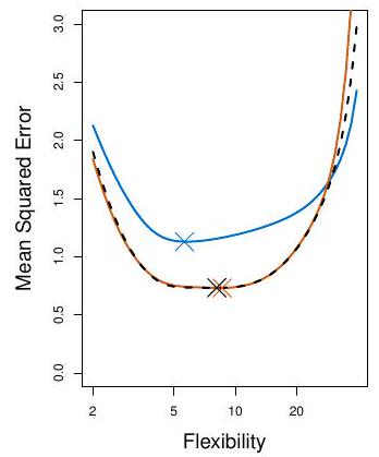
<!-- ## True and estimated test MSE for the simulated data -->
<!--  -->
<!--  -->
<!--  -->
<img data-src="images/clipboard-3294277508.png" class="r-stretch"></section>
<section id="issues-with-cross-validation" class="slide level2">
<h2>Issues with Cross-validation</h2>
<ul>
<li>Since each training set is only <span class="math inline">\((K-1) / K\)</span> as big as the original training set, the estimates of prediction error will typically be biased upward. Why?</li>
<li>This bias is minimized when <span class="math inline">\(K=n\)</span> (LOOCV), but this estimate has high variance, as noted earlier.</li>
<li><span class="math inline">\(K=5\)</span> or 10 provides a good compromise for this bias-variance tradeoff.</li>
</ul>
</section>
<section id="cv-for-classification-problems" class="slide level2">
<h2>CV for Classification Problems</h2>
<div class="font80">
<ul>
<li>Divide the data into <span class="math inline">\(K\)</span> roughly equal-sized parts <span class="math inline">\(C_{1}, C_{2}, \ldots C_{K}\)</span>.</li>
</ul>
<!-- $C_{k}$ denotes the indices of the observations in part $k$. -->
<ul>
<li>There are <span class="math inline">\(n_{k}\)</span> observations in part <span class="math inline">\(k\)</span> and <span class="math inline">\(n_{k}\simeq n / K\)</span>.</li>
<li>Compute <span class="math display">\[
\mathrm{CV}_{K}=\sum_{k=1}^{K} \frac{n_{k}}{n} \operatorname{Err}_{k}
\]</span> where <span class="math inline">\(\operatorname{Err}_{k}=\sum_{i \in C_{k}} I\left(y_{i} \neq \hat{y}_{i}\right) / n_{k}\)</span>.</li>
</ul>
</div>
</section>
<section id="standard-error-of-cv-estimate" class="slide level2">
<h2>Standard error of CV estimate</h2>
<ul>
<li>The estimated standard deviation of <span class="math inline">\(\mathrm{CV}_{K}\)</span> is:</li>
</ul>
<p><span class="math display">\[
\widehat{\mathrm{SE}}\left(\mathrm{CV}_{K}\right)=\sqrt{\frac{1}{K} \sum_{k=1}^{K} \frac{\left(\operatorname{Err}_{k}-\overline{\operatorname{Err}_{k}}\right)^{2}}{K-1}}
\]</span></p>
<ul>
<li>This is a useful estimate, but strictly speaking, not quite valid. Why not?</li>
</ul>
</section>
<section id="why-is-this-an-issue" class="slide level2">
<h2>Why is this an issue?</h2>
<div class="font80">
<ul>
<li><p>In (K)-fold CV, the same dataset is used repeatedly for training and testing across different folds.</p></li>
<li><p>This introduces <strong>correlations</strong> between estimated errors in different folds because each fold’s training set overlaps with others.</p></li>
<li><p>The assumption underlying this estimation of the standard error is that <span class="math inline">\(\operatorname{Err}_{k}\)</span> values are <strong>independent</strong>, which does not hold here.</p></li>
<li><p>The dependence between folds leads to <strong>underestimation</strong> of the true variability in <span class="math inline">\(\mathrm{CV}_K\)</span>, meaning that the reported standard error is likely <strong>too small</strong>, giving a misleading sense of precision in the estimate of the test error.</p></li>
</ul>
</div>
</section>
<section id="cv-right-and-wrong" class="slide level2 scrollable">
<h2>CV: right and wrong</h2>
<!-- - CV needs to be performed the right way beacause it is easy to misunderstand how to do it well. -->
<ul>
<li><p>Consider a classifier applied to some 2-class data:</p>
<ol type="1">
<li>Start with 5000 predictors & 50 samples and find the 100 predictors most correlated with the class labels.</li>
<li>We then apply a classifier such as logistic regression, using only these 100 predictors.</li>
</ol></li>
<li><p>In order to estimate the test set performance of this classifier, <em>¿can we apply cross-validation in step 2, forgetting about step 1?</em></p></li>
</ul>
</section>
<section id="cv-the-wrong-and-the-right-way" class="slide level2">
<h2>CV the Wrong and the Right way</h2>
<div class="font90">
<ul>
<li><p>Applying CV only to Step 2 ignores the fact that in Step 1, the procedure has already used the labels of the training data.</p></li>
<li><p>This is a form of training and <strong>must be included in the validation process</strong>.</p>
<ul>
<li>Wrong way: Apply cross-validation in step 2.</li>
<li>Right way: Apply cross-validation to steps 1 and 2.</li>
</ul></li>
<li><p>This error has happened in many high profile papers, mainly due to a misunderstanding of what CV means and does.</p></li>
</ul>
</div>
</section>
<section id="wrong-way" class="slide level2">
<h2>Wrong Way</h2>
<img data-src="https://cdn.mathpix.com/cropped/2025_02_18_d84fddb1dda73076f5eag-31.jpg?height=503&width=1068&top_left_y=229&top_left_x=101" class="r-stretch"></section>
<section id="right-way" class="slide level2">
<h2>Right Way</h2>
<img data-src="https://cdn.mathpix.com/cropped/2025_02_18_d84fddb1dda73076f5eag-32.jpg?height=499&width=1036&top_left_y=234&top_left_x=112" class="r-stretch"></section>
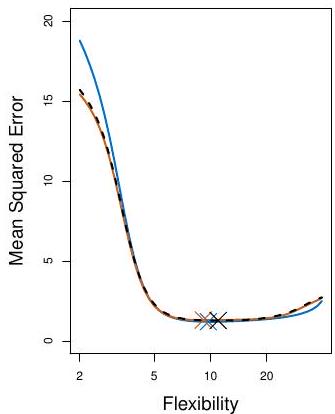
<section id="the-bootstrap" class="slide level2">
<h2>The Bootstrap</h2>
<ul>
<li><p>The bootstrap is a flexible and powerful statistical tool that can be used to quantify the uncertainty associated with a given estimator or statistical learning method.</p></li>
<li><p>For example, it can provide an estimate of the standard error of a coefficient, or a confidence interval for that coefficient.</p></li>
</ul>
<p>… to be continued</p>
<!-- ## Where does the name came from? -->
<!-- - The use of the term bootstrap derives from the phrase to pull -->
<!-- oneself up by one's bootstraps, widely thought to be based on one of -->
<!-- the eighteenth century "The Surprising Adventures of Baron -->
<!-- Munchausen" by Rudolph Erich Raspe: -->
<!-- The Baron had fallen to the bottom of a deep lake. Just when it looked -->
<!-- like all was lost, he thought to pick himself up by his own bootstraps. -->
<!-- - It is not the same as the term "bootstrap" used in computer science -->
<!-- meaning to "boot" a computer from a set of core instructions, though -->
<!-- the derivation is similar. -->
<!-- ## A simple example -->
<!-- - Suppose that we wish to invest a fixed sum of money in two financial -->
<!-- assets that yield returns of $X$ and $Y$, respectively, where $X$ -->
<!-- and $Y$ are random quantities. -->
<!-- - We will invest a fraction $\alpha$ of our money in $X$, and will -->
<!-- invest the remaining $1-\alpha$ in $Y$. -->
<!-- - We wish to choose $\alpha$ to minimize the total risk, or variance, -->
<!-- of our investment. In other words, we want to minimize -->
<!-- $\operatorname{Var}(\alpha X+(1-\alpha) Y)$. -->
<!-- - One can show that the value that minimizes the risk is given by -->
<!-- $$ -->
<!-- \alpha=\frac{\sigma_{Y}^{2}-\sigma_{X Y}}{\sigma_{X}^{2}+\sigma_{Y}^{2}-2 \sigma_{X Y}} -->
<!-- $$ -->
<!-- where -->
<!-- $\sigma_{X}^{2}=\operatorname{Var}(X), \sigma_{Y}^{2}=\operatorname{Var}(Y)$, -->
<!-- and $\sigma_{X Y}=\operatorname{Cov}(X, Y)$. -->
<!-- ## Example continued -->
<!-- - But the values of $\sigma_{X}^{2}, \sigma_{Y}^{2}$, and -->
<!-- $\sigma_{X Y}$ are unknown. -->
<!-- - We can compute estimates for these quantities, -->
<!-- $\hat{\sigma}_{X}^{2}, \hat{\sigma}_{Y}^{2}$, and -->
<!-- $\hat{\sigma}_{X Y}$, using a data set that contains measurements -->
<!-- for $X$ and $Y$. -->
<!-- - We can then estimate the value of $\alpha$ that minimizes the -->
<!-- variance of our investment using -->
<!-- $$ -->
<!-- \hat{\alpha}=\frac{\hat{\sigma}_{Y}^{2}-\hat{\sigma}_{X Y}}{\hat{\sigma}_{X}^{2}+\hat{\sigma}_{Y}^{2}-2 \hat{\sigma}_{X Y}} -->
<!-- $$ -->
<!-- ## Example continued -->
<!--  -->
<!-- Each panel displays 100 simulated returns for investments $X$ and $Y$. -->
<!-- From left to right and top to bottom, the resulting estimates for -->
<!-- $\alpha$ are 0.576, 0.532, 0.657, and 0.651. -->
<!-- ## Example continued -->
<!-- - To estimate the standard deviation of $\hat{\alpha}$, we repeated -->
<!-- the process of simulating 100 paired observations of $X$ and $Y$, -->
<!-- and estimating $\alpha 1,000$ times. -->
<!-- - We thereby obtained 1,000 estimates for $\alpha$, which we can call -->
<!-- $\hat{\alpha}_{1}, \hat{\alpha}_{2}, \ldots, \hat{\alpha}_{1000}$. -->
<!-- - The left-hand panel of the Figure on slide 29 displays a histogram -->
<!-- of the resulting estimates. -->
<!-- - For these simulations the parameters were set to -->
<!-- $\sigma_{X}^{2}=1, \sigma_{Y}^{2}=1.25$, and $\sigma_{X Y}=0.5$, and -->
<!-- so we know that the true value of $\alpha$ is 0.6 (indicated by the -->
<!-- red line). -->
<!-- ## Example continued -->
<!-- - The mean over all 1,000 estimates for $\alpha$ is -->
<!-- $$ -->
<!-- \bar{\alpha}=\frac{1}{1000} \sum_{r=1}^{1000} \hat{\alpha}_{r}=0.5996, -->
<!-- $$ -->
<!-- very close to $\alpha=0.6$, and the standard deviation of the estimates -->
<!-- is -->
<!-- $$ -->
<!-- \sqrt{\frac{1}{1000-1} \sum_{r=1}^{1000}\left(\hat{\alpha}_{r}-\bar{\alpha}\right)^{2}}=0.083 -->
<!-- $$ -->
<!-- - This gives us a very good idea of the accuracy of $\hat{\alpha}$ : -->
<!-- $\mathrm{SE}(\hat{\alpha}) \approx 0.083$. -->
<!-- - So roughly speaking, for a random sample from the population, we -->
<!-- would expect $\hat{\alpha}$ to differ from $\alpha$ by approximately -->
<!-- 0.08 , on average. -->
<!-- ## Results -->
<!--  -->
<!--  -->
<!--  -->
<!-- Left: A histogram of the estimates of $\alpha$ obtained by generating -->
<!-- 1,000 simulated data sets from the true population. Center: A histogram -->
<!-- of the estimates of $\alpha$ obtained from 1,000 bootstrap samples from -->
<!-- a single data set. Right: The estimates of $\alpha$ displayed in the -->
<!-- left and center panels are shown as boxplots. In each panel, the pink -->
<!-- line indicates the true value of $\alpha$. -->
<!-- ## Now back to the real world -->
<!-- - The procedure outlined above cannot be applied, because for real -->
<!-- data we cannot generate new samples from the original population. -->
<!-- - However, the bootstrap approach allows us to use a computer to mimic -->
<!-- the process of obtaining new data sets, so that we can estimate the -->
<!-- variability of our estimate without generating additional samples. -->
<!-- - Rather than repeatedly obtaining independent data sets from the -->
<!-- population, we instead obtain distinct data sets by repeatedly -->
<!-- sampling observations from the original data set with replacement. -->
<!-- - Each of these "bootstrap data sets" is created by sampling with -->
<!-- replacement, and is the same size as our original dataset. As a -->
<!-- result some observations may appear more than once in a given -->
<!-- bootstrap data set and some not at all. -->
<!-- ## Example with just 3 observations -->
<!--  -->
<!-- A graphical illustration of the bootstrap approach on a small sample -->
<!-- containing $n=3$ observations. Each bootstrap data set contains $n$ -->
<!-- observations, sampled with replacement from the original data set. Each -->
<!-- bootstrap data set is used to obtain an estimate of $\alpha$ -->
<!-- - Denoting the first bootstrap data set by $Z^{* 1}$, we use $Z^{* 1}$ -->
<!-- to produce a new bootstrap estimate for $\alpha$, which we call -->
<!-- $\hat{\alpha}^{* 1}$ -->
<!-- - This procedure is repeated $B$ times for some large value of $B$ -->
<!-- (say 100 or 1000), in order to produce $B$ different bootstrap data -->
<!-- sets, $Z^{* 1}, Z^{* 2}, \ldots, Z^{* B}$, and $B$ corresponding -->
<!-- $\alpha$ estimates, -->
<!-- $\hat{\alpha}^{* 1}, \hat{\alpha}^{* 2}, \ldots, \hat{\alpha}^{* B}$. -->
<!-- - We estimate the standard error of these bootstrap estimates using -->
<!-- the formula -->
<!-- $$ -->
<!-- \mathrm{SE}_{B}(\hat{\alpha})=\sqrt{\frac{1}{B-1} \sum_{r=1}^{B}\left(\hat{\alpha}^{* r}-\overline{\hat{\alpha}}^{*}\right)^{2}} -->
<!-- $$ -->
<!-- - This serves as an estimate of the standard error of $\hat{\alpha}$ -->
<!-- estimated from the original data set. See center and right panels of -->
<!-- Figure on slide 29. Bootstrap results are in blue. For this example -->
<!-- $\mathrm{SE}_{B}(\hat{\alpha})=0.087$. -->
<!-- ## A general picture for the bootstrap -->
<!--  -->
<!-- ## The bootstrap in general -->
<!-- - In more complex data situations, figuring out the appropriate way to -->
<!-- generate bootstrap samples can require some thought. -->
<!-- - For example, if the data is a time series, we can't simply sample -->
<!-- the observations with replacement (why not?). -->
<!-- - We can instead create blocks of consecutive observations, and sample -->
<!-- those with replacements. Then we paste together sampled blocks to -->
<!-- obtain a bootstrap dataset. -->
<!-- ## Other uses of the bootstrap -->
<!-- - Primarily used to obtain standard errors of an estimate. -->
<!-- - Also provides approximate confidence intervals for a population -->
<!-- parameter. For example, looking at the histogram in the middle panel -->
<!-- of the Figure on slide 29, the $5 \%$ and $95 \%$ quantiles of the -->
<!-- 1000 values is (.43, .72 ). -->
<!-- - This represents an approximate $90 \%$ confidence interval for the -->
<!-- true $\alpha$. How do we interpret this confidence interval? -->
<!-- - The above interval is called a Bootstrap Percentile confidence -->
<!-- interval. It is the simplest method (among many approaches) for -->
<!-- obtaining a confidence interval from the bootstrap. -->
<!-- ## Can the bootstrap estimate prediction error? -->
<!-- - In cross-validation, each of the $K$ validation folds is distinct -->
<!-- from the other $K-1$ folds used for training: there is no overlap. -->
<!-- This is crucial for its success. Why? -->
<!-- - To estimate prediction error using the bootstrap, we could think -->
<!-- about using each bootstrap dataset as our training sample, and the -->
<!-- original sample as our validation sample. -->
<!-- - But each bootstrap sample has significant overlap with the original -->
<!-- data. About two-thirds of the original data points appear in each -->
<!-- bootstrap sample. Can you prove this? -->
<!-- - This will cause the bootstrap to seriously underestimate the true -->
<!-- prediction error. Why? -->
<!-- - The other way around- with original sample = training sample, -->
<!-- bootstrap dataset $=$ validation sample - is worse! -->
<!-- ## Removing the overlap -->
<!-- - Can partly fix this problem by only using predictions for those -->
<!-- observations that did not (by chance) occur in the current bootstrap -->
<!-- sample. -->
<!-- - But the method gets complicated, and in the end, cross-validation -->
<!-- provides a simpler, more attractive approach for estimating -->
<!-- prediction error. -->
<!-- ## Pre-validation -->
<!-- - In microarray and other genomic studies, an important problem is to -->
<!-- compare a predictor of disease outcome derived from a large number -->
<!-- of "biomarkers" to standard clinical predictors. -->
<!-- - Comparing them on the same dataset that was used to derive the -->
<!-- biomarker predictor can lead to results strongly biased in favor of -->
<!-- the biomarker predictor. -->
<!-- - Pre-validation can be used to make a fairer comparison between the -->
<!-- two sets of predictors. -->
<!-- ## Motivating example -->
<!-- An example of this problem arose in the paper of van't Veer et al. -->
<!-- Nature (2002). Their microarray data has 4918 genes measured over 78 -->
<!-- cases, taken from a study of breast cancer. There are 44 cases in the -->
<!-- good prognosis group and 34 in the poor prognosis group. A "microarray" -->
<!-- predictor was constructed as follows: -->
<!-- 1. 70 genes were selected, having largest absolute correlation with the -->
<!-- 78 class labels. -->
<!-- 2. Using these 70 genes, a nearest-centroid classifier $C(x)$ was -->
<!-- constructed. -->
<!-- 3. Applying the classifier to the 78 microarrays gave a dichotomous -->
<!-- predictor $z_{i}=C\left(x_{i}\right)$ for each case $i$. -->
<!-- ## Results -->
<!-- Comparison of the microarray predictor with some clinical predictors, -->
<!-- using logistic regression with outcome prognosis: -->
<!-- | Model | Coef | Stand. Err. | Z score | p-value | -->
<!-- |:-----------|--------------:|------------:|--------:|--------:| -->
<!-- | Re-use | | | | | -->
<!-- | microarray | 4.096 | 1.092 | 3.753 | 0.000 | -->
<!-- | angio | 1.208 | 0.816 | 1.482 | 0.069 | -->
<!-- | er | -0.554 | 1.044 | -0.530 | 0.298 | -->
<!-- | grade | -0.697 | 1.003 | -0.695 | 0.243 | -->
<!-- | pr | 1.214 | 1.057 | 1.149 | 0.125 | -->
<!-- | age | -1.593 | 0.911 | -1.748 | 0.040 | -->
<!-- | size | 1.483 | 0.732 | 2.026 | 0.021 | -->
<!-- | | Pre-validated | | | | -->
<!-- | | | | | | -->
<!-- | microarray | 1.549 | 0.675 | 2.296 | 0.011 | -->
<!-- | angio | 1.589 | 0.682 | 2.329 | 0.010 | -->
<!-- | er | -0.617 | 0.894 | -0.690 | 0.245 | -->
<!-- | grade | 0.719 | 0.720 | 0.999 | 0.159 | -->
<!-- | pr | 0.537 | 0.863 | 0.622 | 0.267 | -->
<!-- | age | -1.471 | 0.701 | -2.099 | 0.018 | -->
<!-- | size | 0.998 | 0.594 | 1.681 | 0.046 | -->
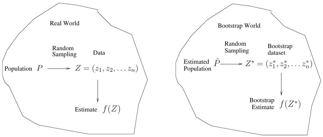
<!-- ## Idea behind Pre-validation -->
<!-- - Designed for comparison of adaptively derived predictors to fixed, -->
<!-- pre-defined predictors. -->
<!-- - The idea is to form a "pre-validated" version of the adaptive -->
<!-- predictor: specifically, a "fairer" version that hasn't "seen" the -->
<!-- response $y$. -->
<!-- ## Pre-validation process -->
<!--  -->
<!-- ## Pre-validation in detail for this example -->
<!-- 1. Divide the cases up into $K=13$ equal-sized parts of 6 cases each. -->
<!-- 2. Set aside one of parts. Using only the data from the other 12 parts, -->
<!-- select the features having absolute correlation at least .3 with the -->
<!-- class labels, and form a nearest centroid classification rule. -->
<!-- 3. Use the rule to predict the class labels for the 13th part -->
<!-- 4. Do steps 2 and 3 for each of the 13 parts, yielding a -->
<!-- "pre-validated" microarray predictor $\tilde{z}_{i}$ for each of the -->
<!-- 78 cases. -->
<!-- 5. Fit a logistic regression model to the pre-validated microarray -->
<!-- predictor and the 6 clinical predictors. -->
<!-- ## The Bootstrap versus Permutation tests -->
<!-- - The bootstrap samples from the estimated population, and uses the -->
<!-- results to estimate standard errors and confidence intervals. -->
<!-- - Permutation methods sample from an estimated null distribution for -->
<!-- the data, and use this to estimate p-values and False Discovery -->
<!-- Rates for hypothesis tests. -->
<!-- - The bootstrap can be used to test a null hypothesis in simple -->
<!-- situations. Eg if $\theta=0$ is the null hypothesis, we check -->
<!-- whether the confidence interval for $\theta$ contains zero. -->
<!-- - Can also adapt the bootstrap to sample from a null distribution (See -->
<!-- Efron and Tibshirani book "An Introduction to the Bootstrap" (1993), -->
<!-- chapter 16) but there's no real advantage over permutations. -->
<div class="quarto-auto-generated-content">
<div class="footer footer-default">
</div>
</div>
</section>
</div>
</div>
<script>window.backupDefine = window.define; window.define = undefined;</script>
<script src="1.3-Model_validation_and_Resampling_files/libs/revealjs/dist/reveal.js"></script>
<!-- reveal.js plugins -->
<script src="1.3-Model_validation_and_Resampling_files/libs/revealjs/plugin/quarto-line-highlight/line-highlight.js"></script>
<script src="1.3-Model_validation_and_Resampling_files/libs/revealjs/plugin/pdf-export/pdfexport.js"></script>
<script src="1.3-Model_validation_and_Resampling_files/libs/revealjs/plugin/reveal-menu/menu.js"></script>
<script src="1.3-Model_validation_and_Resampling_files/libs/revealjs/plugin/reveal-menu/quarto-menu.js"></script>
<script src="1.3-Model_validation_and_Resampling_files/libs/revealjs/plugin/quarto-support/support.js"></script>
<script src="1.3-Model_validation_and_Resampling_files/libs/revealjs/plugin/notes/notes.js"></script>
<script src="1.3-Model_validation_and_Resampling_files/libs/revealjs/plugin/search/search.js"></script>
<script src="1.3-Model_validation_and_Resampling_files/libs/revealjs/plugin/zoom/zoom.js"></script>
<script src="1.3-Model_validation_and_Resampling_files/libs/revealjs/plugin/math/math.js"></script>
<script>window.define = window.backupDefine; window.backupDefine = undefined;</script>
<script>
// Full list of configuration options available at:
// https://revealjs.com/config/
Reveal.initialize({
'controlsAuto': true,
'previewLinksAuto': false,
'pdfSeparateFragments': false,
'autoAnimateEasing': "ease",
'autoAnimateDuration': 1,
'autoAnimateUnmatched': true,
'menu': {"side":"left","useTextContentForMissingTitles":true,"markers":false,"loadIcons":false,"custom":[{"title":"Tools","icon":"<i class=\"fas fa-gear\"></i>","content":"<ul class=\"slide-menu-items\">\n<li class=\"slide-tool-item active\" data-item=\"0\"><a href=\"#\" onclick=\"RevealMenuToolHandlers.fullscreen(event)\"><kbd>f</kbd> Fullscreen</a></li>\n<li class=\"slide-tool-item\" data-item=\"1\"><a href=\"#\" onclick=\"RevealMenuToolHandlers.speakerMode(event)\"><kbd>s</kbd> Speaker View</a></li>\n<li class=\"slide-tool-item\" data-item=\"2\"><a href=\"#\" onclick=\"RevealMenuToolHandlers.overview(event)\"><kbd>o</kbd> Slide Overview</a></li>\n<li class=\"slide-tool-item\" data-item=\"3\"><a href=\"#\" onclick=\"RevealMenuToolHandlers.togglePdfExport(event)\"><kbd>e</kbd> PDF Export Mode</a></li>\n<li class=\"slide-tool-item\" data-item=\"4\"><a href=\"#\" onclick=\"RevealMenuToolHandlers.keyboardHelp(event)\"><kbd>?</kbd> Keyboard Help</a></li>\n</ul>"}],"openButton":true,"width":"half","numbers":true},
'smaller': false,
// Display controls in the bottom right corner
controls: false,
// Help the user learn the controls by providing hints, for example by
// bouncing the down arrow when they first encounter a vertical slide
controlsTutorial: false,
// Determines where controls appear, "edges" or "bottom-right"
controlsLayout: 'edges',
// Visibility rule for backwards navigation arrows; "faded", "hidden"
// or "visible"
controlsBackArrows: 'faded',
// Display a presentation progress bar
progress: true,
// Display the page number of the current slide
slideNumber: 'c/t',
// 'all', 'print', or 'speaker'
showSlideNumber: 'all',
// Add the current slide number to the URL hash so that reloading the
// page/copying the URL will return you to the same slide
hash: true,
// Start with 1 for the hash rather than 0
hashOneBasedIndex: false,
// Flags if we should monitor the hash and change slides accordingly
respondToHashChanges: true,
// Push each slide change to the browser history
history: true,
// Enable keyboard shortcuts for navigation
keyboard: true,
// Enable the slide overview mode
overview: true,
// Disables the default reveal.js slide layout (scaling and centering)
// so that you can use custom CSS layout
disableLayout: false,
// Vertical centering of slides
center: false,
// Enables touch navigation on devices with touch input
touch: true,
// Loop the presentation
loop: false,
// Change the presentation direction to be RTL
rtl: false,
// see https://revealjs.com/vertical-slides/#navigation-mode
navigationMode: 'linear',
// Randomizes the order of slides each time the presentation loads
shuffle: false,
// Turns fragments on and off globally
fragments: true,
// Flags whether to include the current fragment in the URL,
// so that reloading brings you to the same fragment position
fragmentInURL: false,
// Flags if the presentation is running in an embedded mode,
// i.e. contained within a limited portion of the screen
embedded: false,
// Flags if we should show a help overlay when the questionmark
// key is pressed
help: true,
// Flags if it should be possible to pause the presentation (blackout)
pause: true,
// Flags if speaker notes should be visible to all viewers
showNotes: false,
// Global override for autoplaying embedded media (null/true/false)
autoPlayMedia: null,
// Global override for preloading lazy-loaded iframes (null/true/false)
preloadIframes: null,
// Number of milliseconds between automatically proceeding to the